


Next: Wave-Front Propagation
Up: Wave Propagation in Uniform
Previous: Wave Propagation in Magnetized
Let us investigate the propagation of electromagnetic radiation through
a general dispersive medium by studying a simple one-dimensional problem.
Suppose that our dispersive medium extends from  , where it interfaces
with a vacuum, to
, where it interfaces
with a vacuum, to  . Suppose, further, that an electromagnetic wave is incident
normally
on the interface such that the field quantities at the interface only depend on
. Suppose, further, that an electromagnetic wave is incident
normally
on the interface such that the field quantities at the interface only depend on  and
and  .
The wave is then specified as a given function of
at
. Because we are
not interested in the reflected wave, let this function,
.
The wave is then specified as a given function of
at
. Because we are
not interested in the reflected wave, let this function,  , say,
specify the wave amplitude just inside the surface of the dispersive medium.
Suppose that the wave arrives at this surface at
, say,
specify the wave amplitude just inside the surface of the dispersive medium.
Suppose that the wave arrives at this surface at  , and
that
, and
that
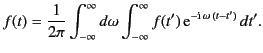
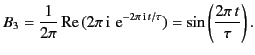
![$\displaystyle f(t) =\left\{\begin{array}{ccl} 0 &\mbox{\hspace{2cm}}& \mbox{for...
...5ex] \sin\!\left(2\pi\, t/\tau\right)&&\mbox{for $t\geq 0$}. \end{array}\right.$](img1771.png) |
(853) |
How does the wave subsequently develop in the region  ? In order to
answer this question, we must first of all decompose
into harmonic
components of the form
? In order to
answer this question, we must first of all decompose
into harmonic
components of the form
 (i.e., Fourier
harmonics). Unfortunately, if we attempt this using only real frequencies,
(i.e., Fourier
harmonics). Unfortunately, if we attempt this using only real frequencies,
 , then we encounter convergence difficulties, because
does not
vanish at
, then we encounter convergence difficulties, because
does not
vanish at  . For the moment, we can circumvent these difficulties
by only considering finite (in time) wave-forms. In other words, we now
imagine that
. For the moment, we can circumvent these difficulties
by only considering finite (in time) wave-forms. In other words, we now
imagine that  for
for  and
and
 . Such a wave-form can be thought
of as the superposition of two infinite (in time) wave-forms, the first
beginning at
, and the second at
. Such a wave-form can be thought
of as the superposition of two infinite (in time) wave-forms, the first
beginning at
, and the second at  with the opposite phase, so
that the two cancel for all time
.
with the opposite phase, so
that the two cancel for all time
.
According to standard Fourier transform theory,
 |
(854) |
Because
is a real function of
that is zero for
and
, we can write
![$\displaystyle f(t) = \frac{1}{2\pi}\int_{-\infty}^{\infty} d\omega \int_0^Tf(t')\,\cos[\omega\,(t-t')]\,dt'.$](img1779.png) |
(855) |
Finally, it follows from symmetry (in
) that
![$\displaystyle f(t) = \frac{1}{\pi}\int_0^{\infty} d\omega \int_0^Tf(t')\,\cos[\omega\,(t-t')]\,dt'.$](img1780.png) |
(856) |
Equation (854) yields
![$\displaystyle f(t) = \frac{1}{\pi}\int_0^{\infty} d\omega \int_0^T \sin\!\left(\frac{2\pi \,t'}{\tau}\right) \,\cos[\omega\,(t-t')]\,dt',$](img1781.png) |
(857) |
or
![$\displaystyle f(t) =\frac{1}{2\pi}\int_0^\infty d\omega\left( \frac{\cos[2\pi \...
...c{\cos[2\pi\, t'/\tau -\omega\,(t-t')]}{\omega+2\pi/\tau}\right)_{t'=0}^{t'=T}.$](img1782.png) |
(858) |
Let us assume, for the sake of simplicity, that
 |
(859) |
where  is a positive integer. This ensures that
is continuous
at
. Equation (859) reduces to
is a positive integer. This ensures that
is continuous
at
. Equation (859) reduces to
![$\displaystyle f(t) = \frac{2}{\tau} \int_0^\infty \frac{d\omega}{\omega^{\,2} -(2\pi/\tau)^{\,2}} \left(\cos[\omega\,(t-T)] -\cos[\omega \,t]\right).$](img1784.png) |
(860) |
This expression can be written
![$\displaystyle f(t) = \frac{1}{\tau} \int_{-\infty}^{\infty} \frac{d\omega}{\omega^{\,2} -(2\pi/\tau)^{\,2}} \left(\cos[\omega\,(t-T)\,] -\cos[\omega \,t]\right),$](img1785.png) |
(861) |
or
![$\displaystyle f(t) = \frac{1}{2\pi}\, {\rm Re}\! \int_{-\infty}^{\infty} \frac{...
...left[ {\rm e}^{-{\rm i}\,\omega\,(t-T)} -{\rm e}^{-{\rm i}\,\omega\, t}\right].$](img1786.png) |
(862) |
It is not entirely obvious that Equation (863) is equivalent to Equation (862).
However, we can easily prove that this is the case by taking Equation (863),
and then using the standard definition of a real part (i.e., half the
sum of the quantity in question and its complex conjugate) to give
![$\displaystyle f(t) = \frac{1}{4\pi} \int_{-\infty}^{\infty} \frac{d\omega}{\ome...
...\left[{\rm e}^{+{\rm i}\,\omega\,(t-T)} -{\rm e}^{+{\rm i}\,\omega \,t}\right].$](img1787.png) |
(863) |
Replacing the dummy integration variable
by  in the
second integral, and then making
use of symmetry, it is easily seen that the previous expression reduces to
Equation (862).
in the
second integral, and then making
use of symmetry, it is easily seen that the previous expression reduces to
Equation (862).
Equation (862) can be written
![$\displaystyle f(t) = \frac{2}{\tau}\int_{-\infty}^{\infty}d\omega\, \sin[\omega\,(t-T/2)]\, \frac{\sin(\omega \,T/2)}{\omega^{\,2} -(2\pi/\tau)^{\,2}}.$](img1789.png) |
(864) |
Note that the integrand is finite at
 , because, at this
point, the vanishing of the denominator is compensated for by the
simultaneous vanishing of the numerator. It follows that the integrand in
Equation (863) is also not infinite at
, as long as we do
not separate the two exponentials. Thus,
we can replace the integration along the real axis through this point by a small semi-circle
in the upper half of the complex plane. Once this has been done, we can deform
the path still further, and can integrate the two exponentials
in Equation (863) separately: that is,
, because, at this
point, the vanishing of the denominator is compensated for by the
simultaneous vanishing of the numerator. It follows that the integrand in
Equation (863) is also not infinite at
, as long as we do
not separate the two exponentials. Thus,
we can replace the integration along the real axis through this point by a small semi-circle
in the upper half of the complex plane. Once this has been done, we can deform
the path still further, and can integrate the two exponentials
in Equation (863) separately: that is,
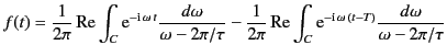 |
(865) |
The contour  is sketched in Figure 6. Note that it runs from
  to
to  , which accounts for the change of sign between Equations (863)
and (866).
, which accounts for the change of sign between Equations (863)
and (866).
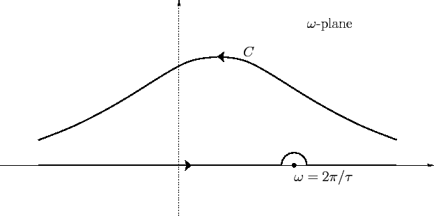
Figure 6:
Sketch of the integration contours used to evaluate
Equations (863) and (866).
 |
We have already mentioned that a finite wave-form that is zero for
and
can be through of as the superposition of two out of phase infinite
wave-forms, one starting at
, and the other at
. It is plausible,
therefore, that the first term in the previous expression corresponds
to the infinite wave form starting at
, and the second to the
infinite wave form starting at
. If this is the case then
the wave-form
(854), which starts at
and ends at
, can be written
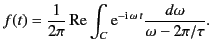 |
(866) |
Let us test this proposition. In order to do this, we must replace the
original path of integration,
, by two equivalent paths.
First, consider
. In this case,
 has a negative
real part in the upper half-plane that increases indefinitely with
increasing distance from the axis. Thus, we can replace the original
path of integration by the path
has a negative
real part in the upper half-plane that increases indefinitely with
increasing distance from the axis. Thus, we can replace the original
path of integration by the path  . (See Figure 7.) If we let
approach infinity in the upper
half-plane then the integral clearly
vanishes along this path. Consequently,
. (See Figure 7.) If we let
approach infinity in the upper
half-plane then the integral clearly
vanishes along this path. Consequently,
 |
(867) |
for
.
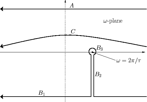
Next, consider  . Now
has a negative
real part in the lower half-plane, so the exponential vanishes at
infinity in this half-plane. If we attempt to deform
to infinity
in the lower half-plane then the path of integration ``catches'' on the
singularity of the integrand at
. (See Figure 7.)
The path of integration
. Now
has a negative
real part in the lower half-plane, so the exponential vanishes at
infinity in this half-plane. If we attempt to deform
to infinity
in the lower half-plane then the path of integration ``catches'' on the
singularity of the integrand at
. (See Figure 7.)
The path of integration  therefore consists of three parts: 1) the
part at infinity,
therefore consists of three parts: 1) the
part at infinity,  , where the integral vanishes due
to the exponential factor
, where the integral vanishes due
to the exponential factor
 ; 2)
; 2)  , the
two parts leading to infinity, which cancel one another, and, thus, contribute
nothing to the integral; 3) the path
, the
two parts leading to infinity, which cancel one another, and, thus, contribute
nothing to the integral; 3) the path  around the singularity. This
latter contribution can easily be evaluated using the Cauchy
residue theorem:
around the singularity. This
latter contribution can easily be evaluated using the Cauchy
residue theorem:
 |
(868) |
Thus, we have proved that expression (867) actually describes a wave-form,
beginning at
, whose subsequent motion is specified by Equation (854).
Figure 7:
Sketch of the integration contours used to evaluate Equation (866).
 |
Equation (867) can immediately be generalized to give the wave motion
in the region
: that is,
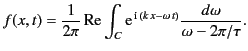 |
(869) |
This follows from standard wave theory, because we know that an
unterminated wave motion at
of the form
takes the form
 after moving a distance
into the dispersive medium, provided that
after moving a distance
into the dispersive medium, provided that  and
are related by the appropriate dispersion relation. For a dielectric medium consisting
of a single resonant species, this dispersion relation is written
[see Equation (785)]
and
are related by the appropriate dispersion relation. For a dielectric medium consisting
of a single resonant species, this dispersion relation is written
[see Equation (785)]
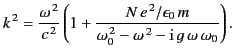 |
(870) |
Next: Wave-Front Propagation
Up: Wave Propagation in Uniform
Previous: Wave Propagation in Magnetized
Richard Fitzpatrick
2014-06-27