


Next: Soft Iron Sphere in
Up: Magnetostatics in Magnetic Media
Previous: Permanent Ferromagnets
Consider a sphere of radius  , with a uniform permanent magnetization
 , surrounded by a vacuum region. The simplest
way of solving this problem is in terms of the scalar magnetic potential
introduced in Equation (701). It follows from Equations (703) and (704)
that
, surrounded by a vacuum region. The simplest
way of solving this problem is in terms of the scalar magnetic potential
introduced in Equation (701). It follows from Equations (703) and (704)
that  satisfies Laplace's equation,
 |
(717) |
because there is zero volume magnetic charge density in a vacuum,
or a uniformly magnetized magnetic medium. However, according to Equation (711),
there is a magnetic surface charge density,
 |
(718) |
on the surface of the sphere. Here,  and
and  are spherical coordinates. One of the matching conditions at the
surface of the sphere is that the tangential component of
are spherical coordinates. One of the matching conditions at the
surface of the sphere is that the tangential component of  must be continuous. It follows from Equation (701) that the scalar magnetic
potential must be continuous at
must be continuous. It follows from Equation (701) that the scalar magnetic
potential must be continuous at  , so that
 |
(719) |
Integrating Equation (703)
over a Gaussian pill-box straddling the surface of the sphere yields
![$\displaystyle \left[\frac{\partial\phi_m}{\partial r}\right]_{r=a-}^{r=a+} = -\sigma_m = -M_0 \cos\theta.$](img1503.png) |
(720) |
In other words, the magnetic charge sheet on the surface of the
sphere gives rise to a discontinuity in the radial gradient of the
magnetic scalar potential at
.
The most general axisymmetric solution to Equation (718) that satisfies physical
boundary conditions at
and  is
is
 |
(721) |
for  , and
, and
 |
(722) |
for  . The boundary condition (720) yields
 |
(723) |
for all  . The boundary condition (721) gives
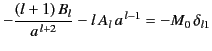 |
(724) |
for all
, because
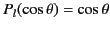 . It follows that
 |
(725) |
for  , and
, and
Thus,
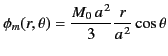 |
(728) |
for
, and
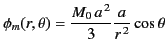 |
(729) |
for
. Because there is a uniqueness theorem associated with
Poisson's equation (see Section 2.3), we can be sure that this axisymmetric potential is
the only solution to the problem that satisfies physical boundary
conditions at  and infinity.
In the vacuum region outside the sphere,
 |
(730) |
It is easily demonstrated from Equation (730) that
![$\displaystyle {\bf B}(r>a) = \frac{\mu_0}{4\pi}\left[ -\frac{{\bf m}}{r^{\,3}} + \frac{3\,({\bf m}\cdot{\bf r})\,{\bf r}}{r^{\,5}} \right],$](img1516.png) |
(731) |
where
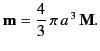 |
(732) |
This, of course, is the magnetic field of a magnetic dipole of moment  . [See Section 5.5.]
Not surprisingly, the net dipole moment of the sphere is equal
to the integral of the magnetization
. [See Section 5.5.]
Not surprisingly, the net dipole moment of the sphere is equal
to the integral of the magnetization  (which is the dipole moment
per unit volume) over the volume of the sphere.
(which is the dipole moment
per unit volume) over the volume of the sphere.
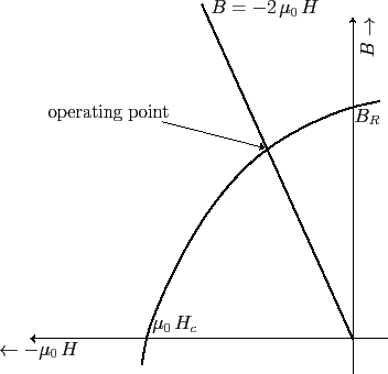
Figure 4:
Schematic demagnetization curve for a permanent magnet.
 |
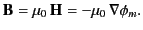
Inside the sphere, we have
 and
and
 , giving
 |
(733) |
and
 |
(734) |
Thus, both the
and  fields are uniform inside the
sphere. Note that the magnetic intensity is oppositely directed to
the magnetization. In other words, the
field
acts to demagnetize the sphere. How successful it is at achieving
this depends on the shape of the hysteresis curve in the negative
fields are uniform inside the
sphere. Note that the magnetic intensity is oppositely directed to
the magnetization. In other words, the
field
acts to demagnetize the sphere. How successful it is at achieving
this depends on the shape of the hysteresis curve in the negative
 and positive
  quadrant. This curve is sometimes called the
demagnetization curve of the magnetic material that makes
up the sphere. Figure 4 shows a schematic demagnetization curve.
The curve is characterized by two quantities: the retentivity
quadrant. This curve is sometimes called the
demagnetization curve of the magnetic material that makes
up the sphere. Figure 4 shows a schematic demagnetization curve.
The curve is characterized by two quantities: the retentivity
 (i.e., the residual magnetic field strength at zero magnetic
intensity) and the coercivity
(i.e., the residual magnetic field strength at zero magnetic
intensity) and the coercivity
 (i.e., the negative
magnetic intensity required to demagnetize the material. The
latter quantity is conventionally multiplied by
(i.e., the negative
magnetic intensity required to demagnetize the material. The
latter quantity is conventionally multiplied by  to give it the
units of magnetic field-strength). The operating point
(i.e., the values of
and
to give it the
units of magnetic field-strength). The operating point
(i.e., the values of
and  inside the sphere)
is obtained from the intersection of the demagnetization curve and
the curve
inside the sphere)
is obtained from the intersection of the demagnetization curve and
the curve
 . It is clear from Equations (734) and (735) that
 |
(735) |
for a uniformly magnetized sphere in the absence of external
fields. The magnetization inside
the sphere is easily calculated once the operating point has been
determined. In fact,
 . It is clear from Figure 4 that
for a magnetic material to be a good permanent magnet it must possess
both a large retentivity and a large coercivity. A material with
a large retentivity but a small coercivity is unable to retain a significant
magnetization in the absence of a strong external magnetizing field.
. It is clear from Figure 4 that
for a magnetic material to be a good permanent magnet it must possess
both a large retentivity and a large coercivity. A material with
a large retentivity but a small coercivity is unable to retain a significant
magnetization in the absence of a strong external magnetizing field.
Next: Soft Iron Sphere in
Up: Magnetostatics in Magnetic Media
Previous: Permanent Ferromagnets
Richard Fitzpatrick
2014-06-27
