 |
(12) |
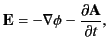
The previous prescription for expressing electric and magnetic fields in terms of the scalar and vector potentials does not
uniquely define the potentials.
Indeed, it can be seen that if
![]() and
and
![]() ,
where
,
where
![]() is an arbitrary scalar field, then the associated electric and magnetic fields are unaffected. The root of the problem lies in the
fact that Equation (11) specifies the curl of the vector potential, but leaves the divergence of this vector field completely
unspecified.
We can make our
prescription unique by adopting a convention that specifies the divergence of the vector potential--such a convention is usually called a gauge condition.
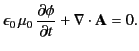
It turns out that Maxwell's equations are Lorentz invariant. (See Chapter 12.) In other words, they take the same form
in all inertial frames. Thus, it makes sense to adopt a gauge condition that is also Lorentz invariant. This leads us
to the so-called Lorenz gauge condition (see Section 12.12),
is an arbitrary scalar field, then the associated electric and magnetic fields are unaffected. The root of the problem lies in the
fact that Equation (11) specifies the curl of the vector potential, but leaves the divergence of this vector field completely
unspecified.
We can make our
prescription unique by adopting a convention that specifies the divergence of the vector potential--such a convention is usually called a gauge condition.
It turns out that Maxwell's equations are Lorentz invariant. (See Chapter 12.) In other words, they take the same form
in all inertial frames. Thus, it makes sense to adopt a gauge condition that is also Lorentz invariant. This leads us
to the so-called Lorenz gauge condition (see Section 12.12),
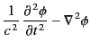
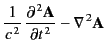
Equations (11)-(13) can be combined with Equations (1) and (4) to give
 |
(16) |