


Next: Exercises
Up: Multipole Expansion
Previous: Spherical Wave Expansion of
Consider a plane electromagnetic wave incident on a spherical
obstacle.
In general, the wave is scattered, to some extent, by the obstacle.
Thus, far away from the sphere, the electromagnetic
fields can be expressed as the sum of a
plane wave and a set of outgoing spherical waves. There may be absorption
by the obstacle, as well as scattering. In this case, the energy
flow away from the obstacle is less than the total energy
flow towards it--the difference representing the absorbed energy.
The fields outside the sphere can be written as the sum of
incident and scattered waves:
where
 and
and
 are given by
(1588)-(1589). Because the scattered fields are outgoing waves
at infinity, their expansions must be of the form
are given by
(1588)-(1589). Because the scattered fields are outgoing waves
at infinity, their expansions must be of the form
The coefficients
 and
and
 are determined
by the boundary conditions on the surface of the sphere. In general,
it is necessary to sum over all
are determined
by the boundary conditions on the surface of the sphere. In general,
it is necessary to sum over all  harmonics in the above expressions. However, for
the restricted class of spherically symmetric scatterers, only the
harmonics in the above expressions. However, for
the restricted class of spherically symmetric scatterers, only the  harmonics need be retained (because only these harmonics occur
in the spherical wave expansion of the incident plane wave [see Equations (1588)-(1589)],
and a spherically symmetric scatterer does not couple different
harmonics).
harmonics need be retained (because only these harmonics occur
in the spherical wave expansion of the incident plane wave [see Equations (1588)-(1589)],
and a spherically symmetric scatterer does not couple different
harmonics).
The angular distribution of
the scattered power can be written in terms
of the coefficients  and
and  using the scattered
electromagnetic
fields evaluated on the surface of a sphere of radius
using the scattered
electromagnetic
fields evaluated on the surface of a sphere of radius
 surrounding the scatterer.
In fact, it is easily demonstrated that
surrounding the scatterer.
In fact, it is easily demonstrated that
![$\displaystyle \frac{d P_{\rm sc}}{d{\mit \Omega}} = \frac{a^{\,2}}{2\,\mu_0} \,...
..., {\rm Re}\,[{\bf E}_{\rm sc}\cdot ({\bf n}\times{\bf B}_{\rm sc}^\ast)]_{r=a},$](img3339.png) |
(1592) |
where  is a radially directed outward normal.
The differential scattering cross-section is defined as the ratio
of
is a radially directed outward normal.
The differential scattering cross-section is defined as the ratio
of
 to the incident flux
 .
Hence,
.
Hence,
![$\displaystyle \frac{d\sigma_{\rm sc}}{d{\mit \Omega}} = - \frac{a^{\,2}}{2} \, ...
...e}\,[{\bf E}_{\rm sc}\cdot ({\bf n}\times c\,{\bf B}_{\rm sc}^{\,\ast})]_{r=a}.$](img3342.png) |
(1593) |
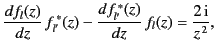
We need
to evaluate this expression using the electromagnetic fields
specified in Equations (1588)-(1593). The
following identity, which can be established with the aid of
Equations (1438), (1476),
and (1486), is helpful in this regard:
![$\displaystyle \nabla\times f(r)\, {\bf X}_{lm} =\frac{{\rm i}\,\sqrt{l\,(l+1)}}...
..._{lm}\, {\bf n}+ \frac{1}{r}\frac{d[r\, f(r)]}{dr}\,{\bf n}\times {\bf X}_{lm}.$](img3343.png) |
(1594) |
For instance, using this result, we can write
 in the form
It can be demonstrated, after considerable algebra, that
![$\displaystyle \frac{d\sigma_{\rm sc}}{d{\mit \Omega}} =\frac{\pi}{2\,k^{\,2}} \...
...rm i}\,\beta_\pm(l)\, {\bf n}\times {\bf X}_{l,\pm 1}\right] \right\vert^{\,2}.$](img3348.png) |
(1596) |
In obtaining this formula, use has been made of the standard result
 |
(1597) |
where
 . The total scattering
cross-section is obtained by integrating Equation (1598) over all solid
angle, making use of the following orthogonality relations
for the vector spherical harmonics [see Equations (1477)-(1478)]:
. The total scattering
cross-section is obtained by integrating Equation (1598) over all solid
angle, making use of the following orthogonality relations
for the vector spherical harmonics [see Equations (1477)-(1478)]:
Thus,
![$\displaystyle \sigma_{\rm sc} = \frac{\pi}{2\,k^{\,2}} \sum_l (2\,l+1)\left[\vert\alpha_\pm(l)\vert^{\,2} +\vert\beta_\pm(l)\vert^{\,2}\right].$](img3354.png) |
(1601) |
According to Equations (1598) and (1603), the total scattering cross-section
is independent of the polarization of the incident radiation (i.e.,
it is the same for both the  signs). However, the differential scattering
cross-section in any particular direction is, in general, different for
different circular polarizations of the incident radiation. This implies
that if the incident radiation is linearly polarized then the scattered radiation
is elliptically polarized. Furthermore, if the incident radiation is
unpolarized then the scattered radiation exhibits partial
polarization, with the degree of polarization depending on
the angle of observation.
signs). However, the differential scattering
cross-section in any particular direction is, in general, different for
different circular polarizations of the incident radiation. This implies
that if the incident radiation is linearly polarized then the scattered radiation
is elliptically polarized. Furthermore, if the incident radiation is
unpolarized then the scattered radiation exhibits partial
polarization, with the degree of polarization depending on
the angle of observation.
The total power absorbed by the sphere is given by
A similar calculation to that outlined above yields the following
expression for the absorption cross-section,
![$\displaystyle \sigma_{\rm abs} = \frac{\pi}{2\,k^{\,2}} \sum_l (2\,l+1)\left[ 2 -\vert\alpha_\pm(l)+1\vert^{\,2} -\vert\beta_\pm(l)+1\vert^{\,2}\right].$](img3356.png) |
(1602) |
The total, or extinction, cross-section is the sum of
 and
and
 :
:
![$\displaystyle \sigma_{\rm t} = -\frac{\pi}{k^{\,2}} \sum_l (2\,l+1) \,{\rm Re}\,[\alpha_\pm(l) +\beta_\pm(l)].$](img3359.png) |
(1603) |
Not surprisingly, the above expressions for the various cross-sections closely
resemble those obtained in quantum mechanics from partial wave expansions.
Let us now consider the boundary conditions at the surface of
the sphere (whose radius is
, say). For the sake of simplicity, let us
suppose that the sphere is a perfect conductor. In this case, the
appropriate boundary condition is that the tangential electric field
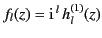
is zero at  . According to Equations (1588), (1590),
and (1596), the tangential electric field is given by
. According to Equations (1588), (1590),
and (1596), the tangential electric field is given by
![$\displaystyle {\bf E}_{\rm tan} = \sum_l {\rm i}^{\,l} \sqrt{4\pi\,(2\,l+1)} \l...
...a_\pm(l)}{2} \,h^{(1)}_l \right)\right] {\bf n}\times{\bf X}_{l,\pm 1}\right\},$](img3360.png) |
(1604) |
where  , and all of the spherical Bessel functions have the argument
 . Thus, the boundary condition yields
where  denotes
  . Note that
 and
and
 are both numbers of modulus unity. This implies, from Equation (1604), that
there is no absorption for the case of a perfectly conducting sphere
(in general, there is some absorption if the sphere has a finite
conductivity). We can write
and
in
the form
are both numbers of modulus unity. This implies, from Equation (1604), that
there is no absorption for the case of a perfectly conducting sphere
(in general, there is some absorption if the sphere has a finite
conductivity). We can write
and
in
the form
where the phase angles  and
and  are called scattering phase shifts. It follows from Equations (1607)-(1608) that
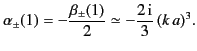
Let us specialize to the limit  , in which the
wavelength of the radiation is much greater than the radius of the sphere.
The asymptotic expansions (1428)-(1429) yield
, in which the
wavelength of the radiation is much greater than the radius of the sphere.
The asymptotic expansions (1428)-(1429) yield
for  .
It is clear that the scattering coefficients
and
become small very rapidly as
.
It is clear that the scattering coefficients
and
become small very rapidly as  increases. Thus, in the
very long wavelength limit, only the
increases. Thus, in the
very long wavelength limit, only the  coefficients need be retained.
It is easily seen that
coefficients need be retained.
It is easily seen that
 |
(1612) |
In this limit, the differential scattering cross-section (1598) reduces
to
 |
(1613) |
It can be demonstrated that
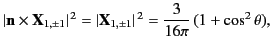 |
(1614) |
and
![$\displaystyle [\pm{\rm i}\,({\bf n}\times{\bf X}_{1,\pm 1}^{\,\ast})\cdot {\bf X}_{1,\pm 1}] = -\frac{3\pi}{8}\,\cos\theta.$](img3386.png) |
(1615) |
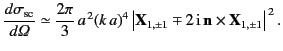
Thus, in long wavelength limit, the differential scattering cross-section
reduces to
![$\displaystyle \frac{d\sigma_{\rm sc}}{d{\mit \Omega}} \simeq a^{\,2} (k\,a)^4\left[ \frac{5}{8}\, (1+\cos^2\theta) -\cos\theta\right].$](img3387.png) |
(1616) |
The scattering is predominately backwards, and is independent of the
state of polarization of the incident radiation. The total scattering
cross-section is given by
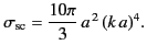 |
(1617) |
This well-known result was first obtained by Mie and Debye. Note that
the cross-section scales as the inverse fourth power of the wavelength
of the incident radiation. This scaling is generic to all scatterers whose
dimensions are much smaller than the wavelength. In fact, it was
first derived by Rayleigh using dimensional analysis.
Next: Exercises
Up: Multipole Expansion
Previous: Spherical Wave Expansion of
Richard Fitzpatrick
2014-06-27
![$\displaystyle \left[ \frac{\,{\rm i}\, \alpha_\pm(l)}{k}\,\frac{1}{r}\frac{d[r ...
...\rm i}\, \beta_\pm(l)\,h_l^{(1)}(k\,r)\,{\bf n}\times {\bf X}_{l,\pm 1}\right].$](img3347.png)
![$\displaystyle P_{\rm abs}= -\frac{a^{\,2}}{2\,\mu_0} \,{\rm Re}\!\int[ {\bf n}\...
... Re}\!\int[{\bf E}\cdot ({\bf n}\times{\bf B}^{\,\ast})]_{r=a}\,d{\mit \Omega}.$](img3355.png)

![$\displaystyle = \left(\frac{[x \,j_l(x)]'} {[x\, y_l(x)]'}\right)_{x=k\,a}.$](img3378.png)
![$\displaystyle \simeq -\frac{2\,{\rm i}\,(k\,a)^{2\,l+1}} {(2\,l+1)\,[(2\,l-1)!!]^{\,2}},$](img3380.png)
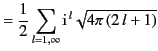
![$\displaystyle = \frac{1}{2}\sum_{l=1,\infty} {\rm i}^{\,l}\sqrt{4\pi\,(2\,l+1)}...
...rac{\beta_\pm(l)}{k}\,\nabla\times h_l^{(1)}(k\,r) \,{\bf X}_{l,\pm 1} \right],$](img3331.png)
![$\displaystyle =\frac{1}{2}\sum_{l=1,\infty} {\rm i}^{\,l}\sqrt{4\pi\,(2\,l+1)} ...
...l,\pm 1} \mp {\rm i}\, \beta_\pm(l)\,h_l^{(1)}(k\,r)\,{\bf X}_{l,\pm 1}\right].$](img3333.png)

![$\displaystyle = -\left(\frac{[x \,h_l^{(2)}(x)]'} {[x\, h_l^{(1)}(x)]'}\right)_{x=k\,a},$](img3365.png)