Next: Time-dependent Maxwell's equations
Up: Time-independent Maxwell equations
Previous: The Biot-Savart law
We have now completed our theoretical
investigation of electrostatics and magnetostatics. Our next task is to incorporate
time variation into our analysis.
However, before we start this, let us briefly review
our progress so far. We have found that the electric fields generated by stationary
charges, and the magnetic fields generated by steady currents, are describable
in terms of four field equations:
The boundary conditions are that the fields are zero at infinity, assuming that
the generating charges and currents are localized
to some region in space. According to Helmholtz's theorem, the above field equations,
plus the boundary conditions, are sufficient to uniquely specify the electric
and magnetic fields. The physical significance of this is that divergence
and curl are the only rotationally invariant first-order differential properties
of a general vector field: i.e., the only quantities which do not change their physical characteristics when the
coordinate axes are rotated. Since physics does not depend on the orientation of the coordinate axes
(which is, after all, quite arbitrary), divergence and curl are the only
quantities which can appear in first-order differential field equations which claim to describe physical
phenomena.
The field equations can be integrated to give:
Here,  is a closed surface enclosing a volume
  . Also,
  is a closed loop,
and
is a closed loop,
and  is some surface attached to this loop. The field equations
(346)-(349) can be deduced
from Eqs. (350)-(353) using Gauss' theorem and Stokes' theorem. Equation
(350) is called Gauss' law, and says that the flux of the electric field
out of a closed surface is proportional to the enclosed electric charge.
Equation (352) has no particular name, and says that there is no such
things as a magnetic monopole. Equation (353) is called Ampère's circuital law,
and says that the line integral of the magnetic
field around any closed loop is proportional
to the flux of the current through the loop. Finally. Eqs. (351) and (353)
are incomplete: each acquires an extra term on the right-hand side in time-dependent situations.
is some surface attached to this loop. The field equations
(346)-(349) can be deduced
from Eqs. (350)-(353) using Gauss' theorem and Stokes' theorem. Equation
(350) is called Gauss' law, and says that the flux of the electric field
out of a closed surface is proportional to the enclosed electric charge.
Equation (352) has no particular name, and says that there is no such
things as a magnetic monopole. Equation (353) is called Ampère's circuital law,
and says that the line integral of the magnetic
field around any closed loop is proportional
to the flux of the current through the loop. Finally. Eqs. (351) and (353)
are incomplete: each acquires an extra term on the right-hand side in time-dependent situations.
The field equation (347) is automatically satisfied if we write
 |
(354) |
Likewise, the field equation (348) is automatically satisfied if we write
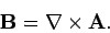 |
(355) |
Here,  is the electric scalar potential, and
  is the magnetic vector
potential. The electric field is clearly unchanged if we add a constant to the
scalar potential:
is the magnetic vector
potential. The electric field is clearly unchanged if we add a constant to the
scalar potential:
 |
(356) |
The magnetic field is similarly unchanged if we add the gradient of a scalar field to
the vector potential:
 |
(357) |
The above transformations, which leave the  and
and  fields
invariant, are called gauge transformations. We are free to choose
fields
invariant, are called gauge transformations. We are free to choose  and
and  to be whatever we like: i.e., we are free to choose the gauge.
The most sensible gauge is the one which make our
equations as simple and symmetric as possible. This corresponds to the choice
to be whatever we like: i.e., we are free to choose the gauge.
The most sensible gauge is the one which make our
equations as simple and symmetric as possible. This corresponds to the choice
 |
(358) |
and
 |
(359) |
The latter convention is known as the Coulomb gauge.
Taking the
divergence of Eq. (354) and the curl of Eq. (355), and making use of the
Coulomb gauge, we find that the four field equations (346)-(349) can be reduced to
Poisson's equation written four times over:
Poisson's equation is just about the simplest rotationally invariant second-order
partial differential equation it is possible to write. Note that
 is clearly rotationally invariant, since it is the divergence of
a gradient, and both divergence and gradient are rotationally invariant.
We can always construct the solution to Poisson's equation, given the
boundary conditions. Furthermore, we have a uniqueness theorem which tells us
that our solution is the only possible solution. Physically, this means that
there is only one electric and magnetic
field which is consistent with a given set of stationary charges and steady currents.
This sounds like an obvious, almost trivial, statement. But there are many
areas of physics (for instance, fluid mechanics and plasma physics) where
we also believe, for physical reasons, that for a given set of boundary conditions
the solution should be unique. The problem is that in most cases
when we reduce the problem to a partial differential equation we end up with
something far nastier than Poisson's equation. In general, we cannot solve
this equation. In fact, we usually cannot even prove that it
possess a solution for general boundary conditions, let alone that the solution
is unique. So, we are very fortunate indeed that
in electrostatics and magnetostatics the problem boils down to solving a
nice partial differential equation. When physicists make statements to the effect that
``electromagnetism is the best understood theory in physics,'' which they often do, what they are really
saying is that the partial differential equations which crop up in this
theory are soluble and have nice properties.
is clearly rotationally invariant, since it is the divergence of
a gradient, and both divergence and gradient are rotationally invariant.
We can always construct the solution to Poisson's equation, given the
boundary conditions. Furthermore, we have a uniqueness theorem which tells us
that our solution is the only possible solution. Physically, this means that
there is only one electric and magnetic
field which is consistent with a given set of stationary charges and steady currents.
This sounds like an obvious, almost trivial, statement. But there are many
areas of physics (for instance, fluid mechanics and plasma physics) where
we also believe, for physical reasons, that for a given set of boundary conditions
the solution should be unique. The problem is that in most cases
when we reduce the problem to a partial differential equation we end up with
something far nastier than Poisson's equation. In general, we cannot solve
this equation. In fact, we usually cannot even prove that it
possess a solution for general boundary conditions, let alone that the solution
is unique. So, we are very fortunate indeed that
in electrostatics and magnetostatics the problem boils down to solving a
nice partial differential equation. When physicists make statements to the effect that
``electromagnetism is the best understood theory in physics,'' which they often do, what they are really
saying is that the partial differential equations which crop up in this
theory are soluble and have nice properties.
Poisson's equation
 |
(362) |
is linear, which means that its solutions are superposable. We can exploit
this fact to construct a general solution to this equation. Suppose that we can
find the solution to
 |
(363) |
which satisfies the boundary conditions.
This is the solution driven by a unit amplitude point source located at position
vector  . Since any general source can be built up out of a weighted sum
of point sources, it follows that a general solution to Poisson's equation
can be built up out of a weighted superposition of point source solutions.
Mathematically, we can write
. Since any general source can be built up out of a weighted sum
of point sources, it follows that a general solution to Poisson's equation
can be built up out of a weighted superposition of point source solutions.
Mathematically, we can write
 |
(364) |
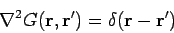
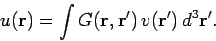
The function  is called the Green's function. The Green's function
for Poisson's equation is
is called the Green's function. The Green's function
for Poisson's equation is
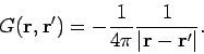 |
(365) |
Note that this Green's function is proportional to the scalar potential of
a point charge located at : this is hardly surprising, given the
definition of a Green's function.
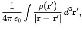
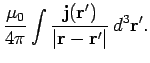
According to Eqs. (360), (361), (362), (364), and (365), the
scalar and vector potentials generated by
a set of stationary charges and steady currents take the form
Making use of Eqs. (354), (355), (366), and (367), we obtain the fundamental force laws for
electric and magnetic fields. Coulomb's law,
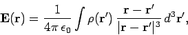 |
(368) |
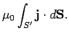
and the Biot-Savart law,
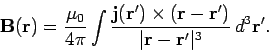 |
(369) |
Of course, both of these laws are examples of action at a distance laws, and,
therefore, violate the theory of relativity. However, this is not a problem as long as we
restrict ourselves to fields generated by
time-independent charge and current distributions.
The question, now, is by how much is this scheme which we have just worked out going to
be disrupted when we take time variation into account. The answer, somewhat
surprisingly, is by very little indeed. So, in Eqs. (346)-(369) we can already
discern the basic outline of classical electromagnetism. Let us continue our
investigation.
Next: Time-dependent Maxwell's equations
Up: Time-independent Maxwell equations
Previous: The Biot-Savart law
Richard Fitzpatrick
2006-02-02