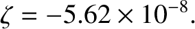
Tidal elongation
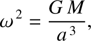
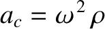
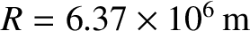
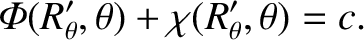
Consider two point masses,  and
and  , executing circular orbits
about their common center of mass,
, executing circular orbits
about their common center of mass,  , with angular
velocity
, with angular
velocity  . Let
. Let  be the distance between
the masses and
be the distance between
the masses and  the distance between point and mass . See Figure 6.6.
We know from Section 4.16 that
the distance between point and mass . See Figure 6.6.
We know from Section 4.16 that
 |
(6.59) |
and
 |
(6.60) |
where 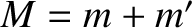 .
.
Figure 6.6:
Two orbiting masses.
|
|
Let us transform to a non-inertial frame of reference that rotates, about an axis perpendicular to the orbital plane and passing through , at
the angular velocity . In this reference frame, both masses appear to be stationary. Consider mass . In the rotating frame, this mass experiences
a gravitational acceleration
 |
(6.61) |
directed toward the center of mass, and a centrifugal acceleration (see Section 6.3)
 |
(6.62) |
directed away from the center of mass.
However, it is easily demonstrated, using Equations (6.59) and (6.60), that
 |
(6.63) |
In other words, the gravitational and centrifugal accelerations
balance, as must be the case if mass is to remain stationary in the
rotating frame. Let us investigate how this balance is affected if the masses and
have finite spatial extents.
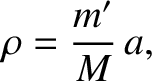
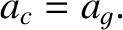
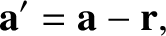
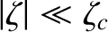
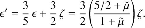
Let the center of the mass distribution lie at  , the center of the
mass distribution at
, the center of the
mass distribution at  , and the center of mass at . See Figure 6.7. We wish to calculate the centrifugal and gravitational
accelerations at some point
, and the center of mass at . See Figure 6.7. We wish to calculate the centrifugal and gravitational
accelerations at some point  in the vicinity of point . It is
convenient to adopt spherical coordinates, centered on point ,
and aligned such that the
in the vicinity of point . It is
convenient to adopt spherical coordinates, centered on point ,
and aligned such that the  -axis coincides with the line
  .
.
Figure 6.7:
Calculation of tidal forces.
|
|
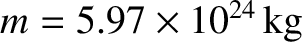
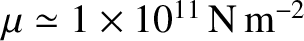
Let us assume that the mass distribution
is orbiting around , but is not rotating about
an axis passing through its center of mass, in order to
exclude rotational flattening from our analysis. If this is the
case then it is easily seen that each constituent point of executes
circular motion of angular velocity and radius . See Figure 6.8. Hence, each point experiences the same
centrifugal acceleration:
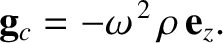 |
(6.64) |
It follows that
 |
(6.65) |
where
 |
(6.66) |
is the centrifugal potential and
 . The centrifugal potential
can also be written
. The centrifugal potential
can also be written
 |
(6.67) |
Figure: 6.8
The center of mass distribution orbits about the center of mass in a circle of radius . If is non-rotating then a noncentral point maintains a constant spatial relationship to , such that orbits some point  that has the same spatial relationship to that has to , in a circle
of radius .
that has the same spatial relationship to that has to , in a circle
of radius .
|
|
The gravitational acceleration at point due to mass is given by
 |
(6.68) |
where the gravitational potential takes the form
 |
(6.69) |
Here,  is the distance between points and . The
gravitational potential generated by the mass distribution is the
same as that generated by an equivalent point mass at , as long
as the distribution is spherically symmetric, which we shall assume to
be the case.
is the distance between points and . The
gravitational potential generated by the mass distribution is the
same as that generated by an equivalent point mass at , as long
as the distribution is spherically symmetric, which we shall assume to
be the case.
Now,
 |
(6.70) |
where  is the vector
 ,
and
,
and  the vector
 . See Figure 6.7.
It follows that
. See Figure 6.7.
It follows that
 |
(6.71) |
Expanding in powers of  , we obtain
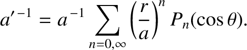 |
(6.72) |
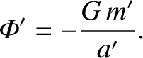
Hence,
![$\displaystyle {\mit\Phi}' \simeq - \frac{G\,m'}{a}\left[1+ \frac{r}{a}\,P_1(\cos\theta) + \frac{r^{\,2}}{a^{\,2}}\,P_2(\cos\theta)\right],$](img1233.png) |
(6.73) |
to second order in , where the  are Legendre polynomials (Abramowitz and Stegun 1965b).
Adding  and
and
 , we find that
![$\displaystyle \chi=\chi'+{\mit\Phi}' \simeq - \frac{G\,m'}{a}\left[1 + \frac{r^{\,2}}{a^{\,2}}\,P_2(\cos\theta)\right],$](img1236.png) |
(6.74) |
to second order in . Note that  is the potential
due to the net externally generated force acting on the mass distribution . This
potential is constant up to first order in , because the first-order
variations in and
cancel each other. The
cancellation
is a manifestation of the balance between the centrifugal and gravitational
accelerations in the equivalent point mass problem discussed previously. However, this balance
is only exact at the center of the mass distribution . Away from the
center, the centrifugal acceleration remains constant, whereas
the gravitational acceleration increases with increasing . At positive , the gravitational
acceleration is larger than the centrifugal acceleration, giving rise to a net acceleration
in the
is the potential
due to the net externally generated force acting on the mass distribution . This
potential is constant up to first order in , because the first-order
variations in and
cancel each other. The
cancellation
is a manifestation of the balance between the centrifugal and gravitational
accelerations in the equivalent point mass problem discussed previously. However, this balance
is only exact at the center of the mass distribution . Away from the
center, the centrifugal acceleration remains constant, whereas
the gravitational acceleration increases with increasing . At positive , the gravitational
acceleration is larger than the centrifugal acceleration, giving rise to a net acceleration
in the  -direction. Likewise, at negative , the centrifugal acceleration
is larger than the gravitational, giving rise to a net acceleration in the
-direction. Likewise, at negative , the centrifugal acceleration
is larger than the gravitational, giving rise to a net acceleration in the  -direction.
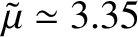
It follows that the mass distribution
is subject to a residual acceleration, represented by the second-order variation in Equation (6.74), that acts to elongate it along the -axis.
This effect is known as tidal elongation.
-direction.
It follows that the mass distribution
is subject to a residual acceleration, represented by the second-order variation in Equation (6.74), that acts to elongate it along the -axis.
This effect is known as tidal elongation.
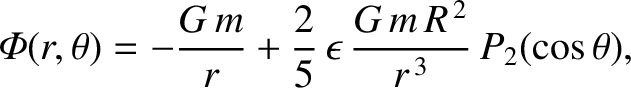
Suppose that
the mass distribution is a sphere of radius  , and uniform density
  , made up of rock similar
to that found in the Earth's mantle.
Let us estimate the elongation of this distribution due to the tidal potential specified in Equation (6.74),
which (neglecting constant terms) can be written
, made up of rock similar
to that found in the Earth's mantle.
Let us estimate the elongation of this distribution due to the tidal potential specified in Equation (6.74),
which (neglecting constant terms) can be written
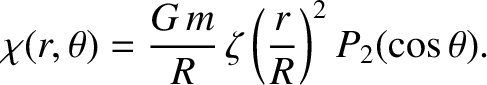 |
(6.75) |
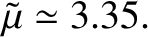
Here, the dimensionless parameter
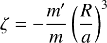 |
(6.76) |
is (minus) the typical ratio of the tidal acceleration to the gravitational acceleration at  .
Let us assume that
.
Let us assume that
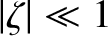 .
By analogy with the analysis in the previous section, in the presence of the tidal potential the
distribution becomes slightly spheroidal in shape, such that its outer boundary satisfies
Equation (6.38). Moreover, the induced ellipticity,
.
By analogy with the analysis in the previous section, in the presence of the tidal potential the
distribution becomes slightly spheroidal in shape, such that its outer boundary satisfies
Equation (6.38). Moreover, the induced ellipticity,  , of the
distribution is related to the normalized amplitude,
, of the
distribution is related to the normalized amplitude,  , of the tidal potential according
to Equation (6.49) if
, of the tidal potential according
to Equation (6.49) if
 , and according to Equation (6.44) if
 .
In the former case, the distribution responds elastically to the tidal potential, whereas in the latter
case it responds like a liquid.
.
In the former case, the distribution responds elastically to the tidal potential, whereas in the latter
case it responds like a liquid.
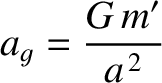
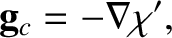
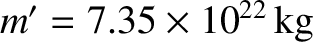
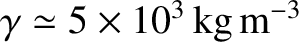
Figure 6.9:
Tidal elongation.
|
|
Consider the tidal elongation of the Earth due to the Moon. In this
case, we have
 ,
,
 ,
,
 , and
, and
 (Yoder 1995).
Hence, we find that
(Yoder 1995).
Hence, we find that
 |
(6.77) |
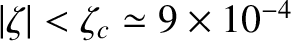
Note that
 . We conclude that the Earth responds elastically to the tidal potential of the Moon, rather
than deforming like a liquid. For the rock that makes up the Earth's mantle,
. We conclude that the Earth responds elastically to the tidal potential of the Moon, rather
than deforming like a liquid. For the rock that makes up the Earth's mantle,
 and
and
 (de Pater and Lissauer 2010). Thus, it follows from Equation (6.50) that
 |
(6.78) |
Hence, according to Equation (6.49), the ellipticity of the Earth
induced by the tidal effect of the Moon is
 |
(6.79) |
The fact that is negative implies that the Earth is elongated along the -axis; that is,
along the axis joining its center to that of the Moon. [See
Equation (6.38).]
If  and
and  are the greatest and least radii of the Earth, respectively, due to this elongation (see Figure 6.9), then
 |
(6.80) |
Thus, we predict that the tidal effect of the Moon (which is actually due to spatial gradients in the Moon's
gravitational field) causes the
Earth to elongate along the axis joining its center to that of the Moon by
about  centimeters. This elongation is only about a quarter of that which would result were the Earth a
non-rigid (i.e., liquid) body.
The true tidal elongation of the Earth due to the Moon is about
centimeters. This elongation is only about a quarter of that which would result were the Earth a
non-rigid (i.e., liquid) body.
The true tidal elongation of the Earth due to the Moon is about  centimeters [assuming a Love number
 (Bertotti et al. 2003)].
We have slightly underestimated this elongation because, for the sake of simplicity, we treated the Earth as a uniform-density body.
(Bertotti et al. 2003)].
We have slightly underestimated this elongation because, for the sake of simplicity, we treated the Earth as a uniform-density body.
Consider the tidal elongation of the Earth due to the Sun. In this case,
we have
,
 ,
, and
,
, and
 .
Hence, we calculate that
.
Hence, we calculate that
 and
and
 , or
, or
 |
(6.81) |
Thus, the tidal elongation of the Earth due to the Sun is about half that due to the Moon. The true tidal elongation of the Earth, due to the Sun, is about  centimeters [assuming a Love number
(Bertotti et al. 2003)].
Again, we have slightly underestimated the elongation because we treated the Earth as a uniform-density body.
centimeters [assuming a Love number
(Bertotti et al. 2003)].
Again, we have slightly underestimated the elongation because we treated the Earth as a uniform-density body.
Because the Earth's oceans are liquid, their tidal elongation
is significantly larger than that of the underlying land. (See Section 6.9, Exercise 9.) Hence,
the oceans rise, relative to the land, in the region of the Earth closest
to the Moon, and also in the region furthest away. Because the Earth
is rotating, while the tidal bulge of the oceans remains relatively
stationary, the Moon's tidal effect causes the ocean at a given point
on the Earth's surface to rise and fall twice daily, giving rise to the
phenomenon known as the tides.
There is also an oceanic tidal bulge due to the Sun that is about half as large as that due to the Moon. Consequently, ocean tides are particularly high when the Sun, the Earth, and
the Moon lie approximately in a straight line, so that the tidal effects of the Sun and the Moon reinforce one another. This occurs at a new moon,
or at a full moon. These type of tides are called spring tides
(the name has nothing to do with the season).
Conversely, ocean
tides are particularly low when the Sun, the Earth, and the Moon
form a right angle, so that the tidal effects of the
Sun and the Moon partially cancel one another. These type of tides are called neap tides. Generally
speaking, we would expect two spring tides and two neap tides per month.
We can roughly calculate the vertical displacement of the oceans, relative to the underlying land, by treating the oceans as a
shallow layer of negligible mass, covering the surface of the Earth. The Earth's external gravitational potential is written
[see Equation (3.65)]
 |
(6.82) |
where is given by Equation (6.79). Let the ocean surface satisfy
![$\displaystyle r = R'(\theta) = R\left[1-\frac{2}{3}\,\epsilon'\,P_2(\cos\theta)\right].$](img1266.png) |
(6.83) |
Because fluids cannot withstand shear stresses, we expect this surface to be an equipotential:
 |
(6.84) |
It follows that, to first order in  and ,
and ,
 |
(6.85) |
Thus, the maximum vertical displacement of the ocean relative to the underlying land is
 |
(6.86) |
As we saw earlier,
 for the Earth. Moreover, the tidal potential due to the Moon is such that
 .
We thus conclude that the Moon causes the oceans to rise a maximum vertical distance of
.
We thus conclude that the Moon causes the oceans to rise a maximum vertical distance of
 relative to the land.
Likewise, the tidal potential due to the Sun is such that
. Hence, we predict that the Sun causes the
oceans to rise a maximum vertical distance of
relative to the land.
Likewise, the tidal potential due to the Sun is such that
. Hence, we predict that the Sun causes the
oceans to rise a maximum vertical distance of
 relative to the land.
In reality, the relationship between ocean tides and the Moon and Sun is much more complicated than that indicated in the previous discussion. This is partly because of the presence of the continents, which impede the flow of the oceanic tidal bulge
around the Earth, and partly because of the finite inertia of the oceans.
Note, finally, that as a consequence of friction within the Earth's crust, and friction between the oceans and the underlying land, there is a time lag of roughly 12 minutes
between the Moon (or Sun) passing directly overhead (or directly below) and
the corresponding maximum in the net tidal elongation of the Earth and the oceans (Bertotti et al. 2003).
![\includegraphics[height=2.75in]{Chapter05/fig5_08.eps}](img1222.png)
![\includegraphics[height=1in]{Chapter05/fig5_06.eps}](img1211.png)
![\includegraphics[height=1.25in]{Chapter05/fig5_07.eps}](img1216.png)
![\includegraphics[height=1.2in]{Chapter05/fig5_09.eps}](img1245.png)