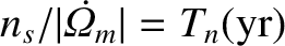
Forced precession and nutation of Earth
This appendix gives a more precise treatment of the precession and nutation of the Earth's axis of rotation, forced by the joint gravitational influence of the Sun and
the Moon, than that presented in Section 8.10.
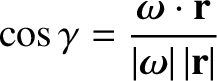
Consider the approximately inertial Cartesian coordinate system,  ,
,  ,
,  , described in Section 8.10.
Let
, described in Section 8.10.
Let
  |
(F.1) |
be the Earth's instantaneous angular velocity vector due to its daily rotation. Here,  is the inclination angle of the Earth's rotation axis to
the normal to the ecliptic plane, whereas
is the inclination angle of the Earth's rotation axis to
the normal to the ecliptic plane, whereas  is the angle subtended between the projection of the rotation axis onto the ecliptic plane and the -axis.
Note that and are Euler angles. (See Section 8.7.)
Suppose that a body of mass
is the angle subtended between the projection of the rotation axis onto the ecliptic plane and the -axis.
Note that and are Euler angles. (See Section 8.7.)
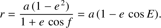
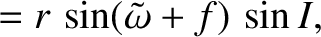
Suppose that a body of mass  is in a Keplerian orbit about the Earth. The coordinates of the body are thus (see Section 4.12)
where
is in a Keplerian orbit about the Earth. The coordinates of the body are thus (see Section 4.12)
where
 |
(F.5) |
Here,
 , and
, and  ,
,  ,
,  ,
,
 ,
,
 ,
,  , and
, and  are the body's orbital major radius, eccentricity, inclination (to the ecliptic), argument of
the perigee, longitude of the ascending node, true anomaly, and eccentric anomaly, respectively. (See Section 4.12.)
are the body's orbital major radius, eccentricity, inclination (to the ecliptic), argument of
the perigee, longitude of the ascending node, true anomaly, and eccentric anomaly, respectively. (See Section 4.12.)
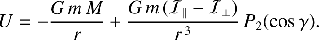
The potential energy of the Earth in the gravitational field of the orbiting body is
 |
(F.6) |
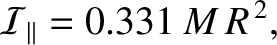
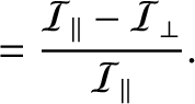
Here,  ,
,
 , and
, and
 are the Earth's mass, moment of inertial about its rotation axis, and moment of
inertia about an axis lying in its equatorial plane, respectively. (See Section 8.10.)
Moreover,
where
are the Earth's mass, moment of inertial about its rotation axis, and moment of
inertia about an axis lying in its equatorial plane, respectively. (See Section 8.10.)
Moreover,
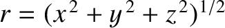
where  is the position vector of the orbiting body.
We are interested in the effect of the orbiting body on the Earth's axis of rotation on timescales that are much longer than the orbital period. We can concentrate on this
effect, and filter out any relatively short-term oscillations, by averaging the potential energy function,  , over an orbital period. In other words,
we replace by
, over an orbital period. In other words,
we replace by
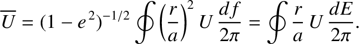 |
(F.8) |
(See Section 10.5.) It follows that
where
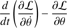
The Earth's orbit-averaged rotational Lagrangian is
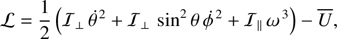 |
(F.12) |
where
 |
(F.13) |
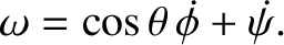
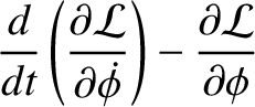
(See Section 8.10.) Here,  is the Earth's third Euler angle. The two non-trivial equations of motion derived
from the preceding Lagrangian are
(The trivial equation merely confirms that the Earth's axial rotation rate,
is the Earth's third Euler angle. The two non-trivial equations of motion derived
from the preceding Lagrangian are
(The trivial equation merely confirms that the Earth's axial rotation rate,  , is a constant.)
Assuming that
, is a constant.)
Assuming that
 , we obtain
Finally, assuming that
, we obtain
Finally, assuming that  at
at  , and also
that
, and also
that
 |
(F.18) |
the lowest-order (in
 ) solutions to Equations (F.16) and (F.17)
are written
where
) solutions to Equations (F.16) and (F.17)
are written
where
 |
 |
(F.21) |
 |
 |
(F.22) |
 |
 |
(F.23) |
 |
 |
(F.24) |
|
 |
(F.25) |
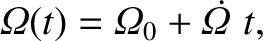
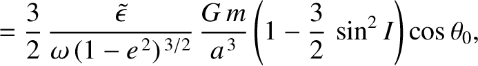
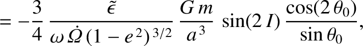
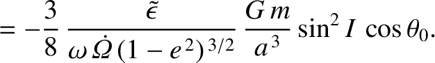
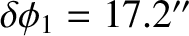
 is the precession rate of the Earth's axis of rotation (a positive rate corresponds to retrograde precession) induced by the orbiting body. Furthermore,
 and
and
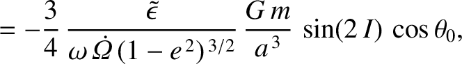
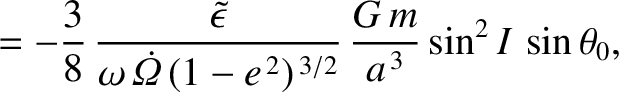
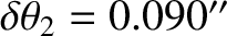
 are the amplitudes of the nutation in the polar angle, , induced by the body. The first amplitude corresponds to nutation
with a period equal to the body's nodal precession period, whereas the second amplitude corresponds to nutation with half this period.
Finally,
are the amplitudes of the nutation in the polar angle, , induced by the body. The first amplitude corresponds to nutation
with a period equal to the body's nodal precession period, whereas the second amplitude corresponds to nutation with half this period.
Finally,
 and
and
 are the corresponding amplitudes of the nutation in the azimuthal angle, .
Note that, in the preceding analysis, there is an implicit assumption that
are the corresponding amplitudes of the nutation in the azimuthal angle, .
Note that, in the preceding analysis, there is an implicit assumption that
 ,
,
 ,
,
 ,
,
 , and, hence,
that
, and, hence,
that
 .
.
The effects of the Sun and the Moon on the Earth's axis of rotation are additive (because the Sun and Moon's gravitational fields are additive).
For the Sun, we can write
where  and
and  are the mean orbital angular velocity, and eccentricity, of the Sun's apparent orbit about the Earth, respectively.
For the Moon, we can write
are the mean orbital angular velocity, and eccentricity, of the Sun's apparent orbit about the Earth, respectively.
For the Moon, we can write
 |
 |
(F.29) |
 |
 |
(F.30) |
 |
 |
(F.31) |
 |
 |
(F.32) |
 ,
,  ,
,  , and
, and
 are the mean orbital angular velocity, eccentricity, inclination (to the ecliptic), and
(negative) nodal precession rate, of the Moon's orbit about the Earth, respectively.
Furthermore,
are the mean orbital angular velocity, eccentricity, inclination (to the ecliptic), and
(negative) nodal precession rate, of the Moon's orbit about the Earth, respectively.
Furthermore,
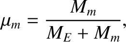 |
(F.33) |
where  and
and  are the masses of the Moon and Earth, respectively.
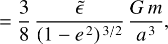
The net luni-solar precession rate of the Earth's rotation axis (which is the sum of the precession rates due to the Sun and the Moon) is written
![$\displaystyle {\mit\Omega}_\phi = \frac{3}{2}\,\frac{\skew{3}\tilde{\epsilon}\,...
...\,\mu_m}{(1-e_m^{\,2})^{\,3/2}}
\,\left(1-\frac{3}{2}\,\sin^2 I_m\right)\right]$](img4589.png) |
(F.34) |
Now,
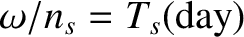 ,
,
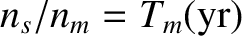 , and
, and
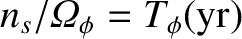 , where
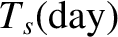 is the number of stellar (sidereal) days in a sidereal year,
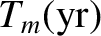 is the length of a sidereal month in units of sidereal years,
and
is the length of a sidereal month in units of sidereal years,
and
 is the precession period of the Earth's axis of rotation in sidereal years. Thus,
![$\displaystyle T_\phi({\rm yr}) = \frac{2}{3}\,\frac{T_s({\rm day})}{\skew{3}\ti...
...r})]^{\,2}}\,
\frac{[1-(3/2)\,\sin^2 I_m]}{(1-e_m^{\,2})^{\,3/2}}\right\}^{-1}.$](img4596.png) |
(F.35) |
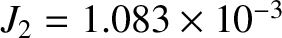
Using the following observed values,
 ,
,
 ,
,
 ,
,
 ,
,
 ,
,
 , and
, and
 , (Yoder 1995)
we obtain
, (Yoder 1995)
we obtain
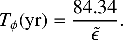 |
(F.36) |
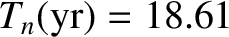
In fact, the observed precession period of the Earth's axis of rotation is
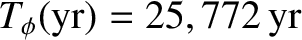 (Yoder 1995). This suggests that the Earth's dynamical
ellipticity,
, which cannot be measured directly, takes the value
(Yoder 1995). This suggests that the Earth's dynamical
ellipticity,
, which cannot be measured directly, takes the value
 |
(F.37) |
(In fact, this is how the Earth's dynamical ellipticity is most accurately determined.)
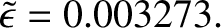
The previous value is less than the value,
 , used in Section 8.10, which was derived from the Earth's observed flattening on the simplistic assumption that it is a homogeneous body. [See Equation (8.95).]
We can write
, used in Section 8.10, which was derived from the Earth's observed flattening on the simplistic assumption that it is a homogeneous body. [See Equation (8.95).]
We can write
 |
(F.38) |
where  is the Earth's equatorial radius, and
 is its measured dimensionless gravitational quadrupole moment. (See Section 10.5.)
Thus, we deduce that
is its measured dimensionless gravitational quadrupole moment. (See Section 10.5.)
Thus, we deduce that
 |
(F.39) |
which confirms that the Earth's internal mass distribution is not homogeneous (because, if it were then
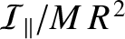 would
take the value
would
take the value  ), but is instead centrally concentrated. In fact, the previous value for
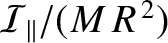 is very similar to
that predicted by the so-called Darwin-Radau equation. (See Appendix D.) This suggests that the
Earth's response to its centrifugal potential is essentially fluid-like.
is very similar to
that predicted by the so-called Darwin-Radau equation. (See Appendix D.) This suggests that the
Earth's response to its centrifugal potential is essentially fluid-like.
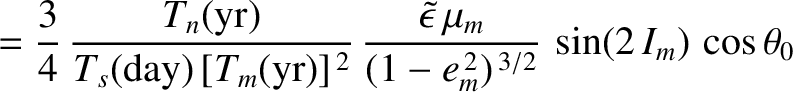
Now,
 , where
 is the Moon's observed nodal precession period in sidereal
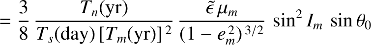
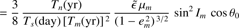
years (Yoder 1965). Thus, making use of the deduced value, given in Equation (F.37), for the Earth's dynamical ellipticity, we find that the nutation amplitudes induced by the Moon are
is the Moon's observed nodal precession period in sidereal
years (Yoder 1965). Thus, making use of the deduced value, given in Equation (F.37), for the Earth's dynamical ellipticity, we find that the nutation amplitudes induced by the Moon are
|
 |
|
| |
 |
(F.40) |
|
 |
|
| |
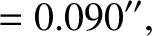 |
(F.41) |
|
 |
|
| |
 |
(F.42) |
 |
 |
|
| |
 |
(F.43) |
 .)
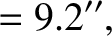
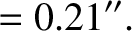
The observed nutation amplitudes are
.)
The observed nutation amplitudes are
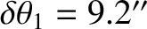 ,
,
 ,
,
 , and
, and
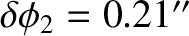 (Meeus 2005).
The fact that the calculated nutation amplitudes agree so well with the observed amplitudes validates our general approach.
(Meeus 2005).
The fact that the calculated nutation amplitudes agree so well with the observed amplitudes validates our general approach.

![$\displaystyle = r\left[\cos{\mit\Omega}\,\cos(\tilde{\omega}+f)-\sin{\mit\Omega}\,\sin(\tilde{\omega}+f)\,\cos I\right],$](img4528.png)

![$\displaystyle = r\left[\sin{\mit\Omega}\,\cos(\tilde{\omega}+f)+\cos{\mit\Omega}\,\sin(\tilde{\omega}+f)\,\cos I\right],$](img4529.png)


![$\displaystyle \phantom{=}+ \sin(\tilde{\omega}+f)\left[\cos I\,\sin\theta\,\cos({\mit\Omega}-\phi)+\sin I\,\cos\theta\right],$](img4536.png)


![$\displaystyle \phantom{=}\left. + \sin(2\,I)\,\sin(2\,\theta)\,\cos ({\mit\Omega}-\phi)
-\sin^2 I\, \sin^2\theta\,\cos[2\,({\mit\Omega}-\phi)]\right\},$](img4540.png)


![$\displaystyle \simeq -2\,\alpha\,[1-(3/2)\,\sin^2 I]\,\sin(2\,\theta)-2\,\alpha\,\sin(2\,I)\,\cos(2\,\theta)\,\cos({\mit\Omega}-\phi)$](img4549.png)
![$\displaystyle \phantom{=}+ \alpha\,\sin^2 I\,\sin(2\,\theta)\,\cos[2\,({\mit\Omega}-\phi)],$](img4550.png)
![$\displaystyle \simeq \alpha\,\sin(2\,I)\,\sin(2\,\theta)\,\sin({\mit\Omega}-\phi)-2\,\alpha\,\sin^2 I\,\sin^2\theta\,\sin[2\,({\mit\Omega}-\phi)].$](img4552.png)

![$\displaystyle = -{\mit\Omega}_\phi\,t +\delta\phi_1\left(\sin{\mit\Omega}-\sin{...
...ght) - \delta\phi_2
\left[\sin(2\,{\mit\Omega})-\sin(2\,{\mit\Omega}_0)\right],$](img4555.png)