


Next: Schrödinger Wave Equation
Up: Quantum Dynamics
Previous: Heisenberg Equation of Motion
We have now introduced all of the basic elements of quantum mechanics. The only
thing which is lacking is some rule to determine the form of the
quantum mechanical Hamiltonian. For a physical system that possess a classical
analogue, we generally assume that the Hamiltonian has the same form as
in classical physics (i.e., we replace the classical coordinates and conjugate
momenta by the corresponding quantum mechanical operators). This scheme guarantees
that quantum mechanics yields the correct classical equations of motion
in the classical limit. Whenever an ambiguity arises because of
non-commuting
observables, this can usually be resolved by requiring the Hamiltonian  to
be an Hermitian operator. For instance, we would write the
quantum mechanical analogue of the classical product
to
be an Hermitian operator. For instance, we would write the
quantum mechanical analogue of the classical product  , appearing in the
Hamiltonian, as the Hermitian product
, appearing in the
Hamiltonian, as the Hermitian product
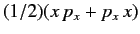 . When the system
in question has no classical analogue then we are reduced to guessing a form
for
that reproduces the observed behavior of the system.
. When the system
in question has no classical analogue then we are reduced to guessing a form
for
that reproduces the observed behavior of the system.
Consider a three-dimensional system characterized by three independent Cartesian
position coordinates  (where
  runs from 1 to 3), with three corresponding
conjugate momenta
runs from 1 to 3), with three corresponding
conjugate momenta  . These are represented by three commuting position
operators
, and three commuting momentum operators
, respectively. The
commutation
relations satisfied by the position and momentum operators
are [see Equation (116)]
. These are represented by three commuting position
operators
, and three commuting momentum operators
, respectively. The
commutation
relations satisfied by the position and momentum operators
are [see Equation (116)]
![$\displaystyle [x_i, p_j] = {\rm i}\,\hbar\, \delta_{ij}.$](img586.png) |
(251) |
It is helpful to denote
 as
as  and
and
 as
as
 . The following useful formulae,
where
 and
and
 are functions that can be expanded as power series, are
easily proved using the fundamental commutation relations, (251).
are functions that can be expanded as power series, are
easily proved using the fundamental commutation relations, (251).
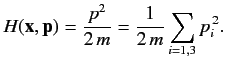
Let us now consider the three-dimensional motion of a free particle of mass
 in the
Heisenberg picture. The Hamiltonian is assumed to have the same form as in
classical physics: i.e.,
in the
Heisenberg picture. The Hamiltonian is assumed to have the same form as in
classical physics: i.e.,
 |
(254) |
In the following, all dynamical variables are assumed to be Heisenberg dynamical
variables, although we will omit the subscript  for the sake of clarity.
The time evolution of the momentum operator
follows from the Heisenberg
equation of motion, (244). We find that
for the sake of clarity.
The time evolution of the momentum operator
follows from the Heisenberg
equation of motion, (244). We find that
![$\displaystyle \frac{dp_i}{dt} = \frac{1}{{\rm i}\,\hbar}\,[p_i, H] = 0,$](img599.png) |
(255) |
since
automatically commutes with any function of the momentum operators.
Thus, for a free particle, the momentum operators are constants of the motion,
which means that
 at all times
(for
is 1 to 3).
The time evolution of the position operator
is given by
at all times
(for
is 1 to 3).
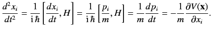
The time evolution of the position operator
is given by
![$\displaystyle \frac{d x_i}{dt} = \frac{1}{{\rm i}\,\hbar}\, [x_i, H] = \frac{1}...
... p_i}\! \left(\sum_{j=1,3} p_j^{\,2}\right) = \frac{p_i}{m} = \frac{p_i(0)}{m},$](img601.png) |
(256) |
where use has been made of Equation (252). It follows that
![$\displaystyle x_i(t) = x_i(0) + \left[\frac{p_i(0)}{m}\right] t,$](img602.png) |
(257) |
which is analogous to the equation of motion of a classical free particle.
Note that even though
![$\displaystyle [x_i(0), x_j(0)] = 0,$](img603.png) |
(258) |
where the position operators are evaluated at equal times, the
do not
commute when evaluated at different times. For instance,
![$\displaystyle [x_i(t), x_i(0)] = \left[ \frac{p_i(0)\,t}{m}, x_i(0)\right] = \frac{-{\rm i}\,\hbar \,t} {m}.$](img604.png) |
(259) |
Combining the above commutation relation with the uncertainty relation (83) yields
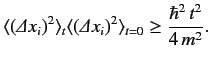 |
(260) |
This result implies that even if a particle is well-localized at  , its
position becomes progressively more uncertain with time. This conclusion
can also be obtained by studying the propagation of wavepackets in
wave mechanics.
, its
position becomes progressively more uncertain with time. This conclusion
can also be obtained by studying the propagation of wavepackets in
wave mechanics.
Let us now add a potential
 to our free particle Hamiltonian:
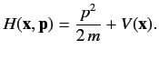 |
(261) |
Here,  is some (real) function of the
operators. The Heisenberg equation of
motion gives
is some (real) function of the
operators. The Heisenberg equation of
motion gives
![$\displaystyle \frac{d p_i}{dt} = \frac{1}{{\rm i}\,\hbar} \,[p_i, V({\bf x})] = - \frac{\partial V({\bf x})}{\partial x_i},$](img610.png) |
(262) |
where use has been made of Equation (253). On the other hand, the result
 |
(263) |
still holds, because the
all commute with the new term,
, in the
Hamiltonian. We can use the Heisenberg equation of motion a second time
to deduce that
 |
(264) |
In vectorial form, this equation becomes
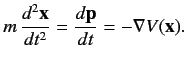 |
(265) |
This is the quantum mechanical equivalent of Newton's second law of motion.
Taking the expectation values of both sides with respect to a Heisenberg
state ket that does not evolve in time, we obtain the so-called Ehrenfest theorem:
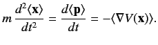 |
(266) |
When written in terms of expectation
values, this result is independent of whether we are using the Heisenberg or
Schrödinger picture. By contrast, the operator equation (265) only holds
if
and
are understood to be Heisenberg dynamical variables.
Note that Equation (266) has no dependence on  .
In fact, it guarantees to us that the centre of
a wavepacket always moves like a classical particle.
.
In fact, it guarantees to us that the centre of
a wavepacket always moves like a classical particle.
Next: Schrödinger Wave Equation
Up: Quantum Dynamics
Previous: Heisenberg Equation of Motion
Richard Fitzpatrick
2013-04-08

