Next: Hydrogen Molecule Ion
Up: Identical Particles
Previous: Orthohelium and Parahelium
Variational Principle
Suppose that we wish to find an approximate solution to the time-independent Schrödinger equation,
 |
(9.68) |
where  is a known (presumably complicated) time-independent Hamiltonian, and
  the energy eigenvalue.
Let
the energy eigenvalue.
Let
 be a properly normalized trial solution to the above equation that corresponds to the trial wavefunction
 .
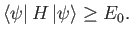
The so-called variational principle [94] states, quite simply, that the
ground-state energy,
.
The so-called variational principle [94] states, quite simply, that the
ground-state energy,  , is always less than, or equal to, the expectation
value of
calculated with the trial solution: that is,
, is always less than, or equal to, the expectation
value of
calculated with the trial solution: that is,
 |
(9.69) |
Thus, by varying
until the expectation value of
is minimized, we can
obtain approximations to both the energy and the wavefunction of the ground state.
(Incidentally, if
is not properly normalized then we must minimize
 . See Exercise 16.)
Let us prove the variational principle.
Suppose that the  and the
  are the true eigenvalues and eigenkets
of
: that is,
are the true eigenvalues and eigenkets
of
: that is,
 |
(9.70) |
Furthermore, let
 |
(9.71) |
so that  is the ground state,
  the first excited state,
et cetera. The
are assumed to be orthonormal:
that is,
the first excited state,
et cetera. The
are assumed to be orthonormal:
that is,
 |
(9.72) |
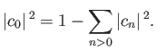
If our trial ket
is properly normalized then
we can write
 |
(9.73) |
where
 |
(9.74) |
and the  are complex numbers.
Here,
are complex numbers.
Here,  is summed from 0
to
is summed from 0
to  .
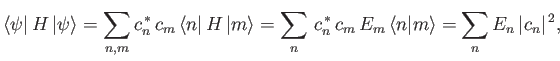
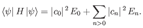
Now, the expectation value of
, calculated with
, takes the
form
.
Now, the expectation value of
, calculated with
, takes the
form
 |
(9.75) |
where use has been made of Equations (9.71), (9.73), and (9.74).
So, we can write
 |
(9.76) |
However, Equation (9.75) can be rearranged to give
 |
(9.77) |
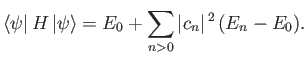
Combining the previous two equations, we obtain
 |
(9.78) |
But, the second term on the right-hand side of the previous expression
is positive definite, because  for all
  . [See Equation (9.72).]
Hence, we obtain the desired result:
. [See Equation (9.72).]
Hence, we obtain the desired result:
 |
(9.79) |
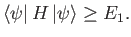
If
is a properly normalized trial ket that is
orthogonal to the true ground-state of the system (i.e.,
 )
then, by repeating the previous analysis, we can easily demonstrate that
)
then, by repeating the previous analysis, we can easily demonstrate that
 |
(9.80) |
Thus, by varying
until the expectation value of
is minimized, we can
obtain approximations to both the energy and wavefunction of the first excited state. In reality, because we
do not generally know the exact ground state, we have to use a trial ket that is orthogonal
to the approximate ground state obtained via the variational method described in the preceding paragraph.
Obviously, we can continue this process until we have approximations
to all of the stationary eigenstates. Note, however, that the errors are clearly cumulative in this approach,
so that any approximations to highly excited states are likely to inaccurate. For this reason, the variational method is generally
used only to calculate the ground state, and the first few excited states, of
complicated quantum systems.
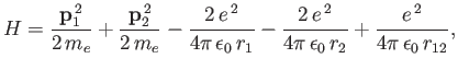
We can employ the variational principle to obtain an improved estimate for the ground-state energy of a helium atom.
The Hamiltonian is written [see Equation (9.52)]
 |
(9.81) |
where we have now explicitly taken into account the fact that the nuclear charge is  . Let us
take [see Equation (9.54)]
. Let us
take [see Equation (9.54)]
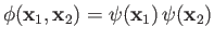 |
(9.82) |
as our properly normalized trial wavefunction, where [see Equation (9.56)]
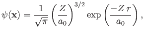 |
(9.83) |
and  is the Bohr radius.
In the following, we shall treat
is the Bohr radius.
In the following, we shall treat  as a variable parameter. In fact,
  is the nuclear charge experienced by each
electron. We would expect this quantity to be somewhat less that the true nuclear charge,
, because the
electrons partially shield one another from the nucleus.
is the nuclear charge experienced by each
electron. We would expect this quantity to be somewhat less that the true nuclear charge,
, because the
electrons partially shield one another from the nucleus.
It is convenient to rewrite the Hamiltonian in the form
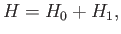 |
(9.84) |
where
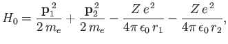 |
(9.85) |
and
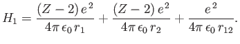 |
(9.86) |
The trial wavefunction, (9.83), is an exact eigenstate of  belonging to the eigenvalue
 ,
where
is the ground-state energy of hydrogen. [See Equation (9.57).] If we treat
,
where
is the ground-state energy of hydrogen. [See Equation (9.57).] If we treat  as a perturbation (see Chapter 7) then we obtain
the estimate
as a perturbation (see Chapter 7) then we obtain
the estimate
 |
(9.87) |
for the ground-state energy of helium. Here, the expectation value is calculated using the
trial wavefunction.
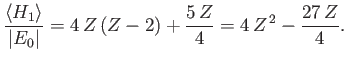
Given that
 , we get
![$\displaystyle \langle H_1\rangle= \left[2\,(Z-2)\left\langle\frac{a_0}{r_1}\rig...
...ght\rangle + 2\left\langle\frac{a_0}{r_{12}}\right\rangle\right]\vert E_0\vert.$](img3185.png) |
(9.88) |
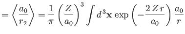
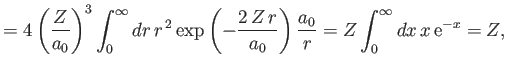
However, we already proved in Section 9.5 that
 |
(9.89) |
[See Equations (9.58) and (9.63).]
Furthermore,
where
 , and use has been made of Exercise 11. Thus,
 |
(9.91) |
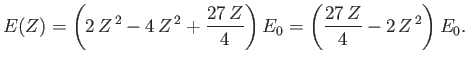
According to the previous analysis, when expressed as a function of
, the ground-state energy of a helium atom takes the form
 |
(9.92) |
We must now minimize this expression with respect to
to obtain our new estimate for the
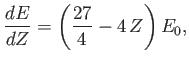
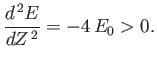
actual ground-state energy. It is easily seen that
 |
(9.93) |
and
 |
(9.94) |
Thus,
clearly attains a minimum value when
 |
(9.95) |
The fact that  confirms our earlier conjecture that the electrons partially shield the
nuclear charge from one another. Our new estimate for the ground-state energy of helium is [68]
confirms our earlier conjecture that the electrons partially shield the
nuclear charge from one another. Our new estimate for the ground-state energy of helium is [68]
 |
(9.96) |
This is clearly an improvement on our previous estimate,
 [see Equation (9.64)], recalling that the correct
result is
[see Equation (9.64)], recalling that the correct
result is
 [75].
[75].
Next: Hydrogen Molecule Ion
Up: Identical Particles
Previous: Orthohelium and Parahelium
Richard Fitzpatrick
2016-01-22