Next: Electric Quadrupole Transitions
Up: Time-Dependent Perturbation Theory
Previous: Forbidden Transitions
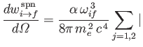
According to Equation (8.195), the quantity that mediates spontaneous magnetic dipole
transitions between different atomic states is
 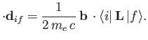 |
(8.194) |
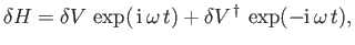
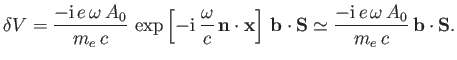
However, it turns out that the previous expression is incomplete because, in writing the Hamiltonian (8.128), we neglected
to take into account the interaction of the magnetic component of the electromagnetic wave with the electron's magnetic
moment. This interaction gives rise to an additional term [49]
where  is the electron spin. (See Section 5.5.)
Now,
is the electron spin. (See Section 5.5.)
Now,
 |
(8.196) |
where

 , and use has been made of Equation (8.130). It follows that
 |
(8.197) |
where
 |
(8.198) |
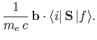
Hence, according to Equation (8.137), there is an addition contribution to
 of the
form
of the
form
 |
(8.199) |
(Here, we have again assumed that
 .)
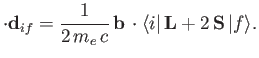
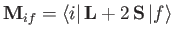
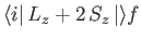
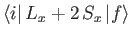
In other words, the complete quantity that mediates magnetic dipole transitions between different atomic states is
.)
In other words, the complete quantity that mediates magnetic dipole transitions between different atomic states is
 |
(8.200) |
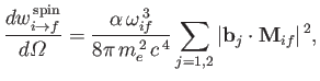
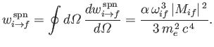
It follows, by analogy with Equation (8.165), that the spontaneous emission rate associated
with a magnetic dipole transition is
 |
(8.201) |
where
 |
(8.202) |
is termed the magnetic dipole matrix element,
and

 . Here,
 is the solid angle associated with the
direction of the
emitted photon's normalized wavevector,
is the solid angle associated with the
direction of the
emitted photon's normalized wavevector,  . Moreover,
are the photon's two independent electric polarization vectors.
In fact, it is easily demonstrated that
. Moreover,
are the photon's two independent electric polarization vectors.
In fact, it is easily demonstrated that

 , and
, and

 .
Hence, Equation (8.204) can also be written
.
Hence, Equation (8.204) can also be written
It follows that
 |
(8.204) |
(See Exercise 8.)
According to the analysis of Chapters 4 and 5,
 is only non-zero
for a hydrogen-like atom if
is only non-zero
for a hydrogen-like atom if
 ,
,
 , and
, and
 . Here,
 is the azimuthal quantum number,
  the magnetic quantum number, and
  the spin quantum number. Likewise,
 and
and
 are only non-zero if
,
are only non-zero if
,
 , and
, and
 .
Hence, the selection rules for magnetic dipole transitions are
.
Hence, the selection rules for magnetic dipole transitions are
Consider the hydrogen atom.
Let us calculate the magnetic dipole matrix element,
 , for the case where the initial state is characterized by the
quantum numbers
, for the case where the initial state is characterized by the
quantum numbers  ,
,
, and
, and the final state is characterized by the
quantum numbers
,
,
, and
, and the final state is characterized by the
quantum numbers  ,
,  ,
,  , and
, and  . Because
 has no
dependance on the radial variable
has no
dependance on the radial variable  , the radial component of this matrix element is simply
 |
(8.208) |
where  is a standard hydrogen radial wavefunction. Here, we have made use of the
fact that the matrix element is zero unless
is a standard hydrogen radial wavefunction. Here, we have made use of the
fact that the matrix element is zero unless  . However, according to Exercise 17, the
previous integral is zero unless
. However, according to Exercise 17, the
previous integral is zero unless  : that is, unless the initial and final states have the same energy.
Hence, we conclude that magnetic dipole transitions
between different energy levels (i.e., atomic states corresponding to different values of the principle quantum number,
) of a hydrogen atom are forbidden.
: that is, unless the initial and final states have the same energy.
Hence, we conclude that magnetic dipole transitions
between different energy levels (i.e., atomic states corresponding to different values of the principle quantum number,
) of a hydrogen atom are forbidden.
A more general form of the selection rules (8.208)-(8.210) is [23]
where  and
and  are the standard quantum numbers associated with the total angular
momentum of the system. Note, however, that a magnetic
dipole transition between two
are the standard quantum numbers associated with the total angular
momentum of the system. Note, however, that a magnetic
dipole transition between two  states is forbidden. These new rules suggest that it is possible to have a magnetic
dipole transition between hydrogen atom states whose energies are split by
spin-orbit effects: for instance, between a
states is forbidden. These new rules suggest that it is possible to have a magnetic
dipole transition between hydrogen atom states whose energies are split by
spin-orbit effects: for instance, between a
 and a
and a
 state. (See Section 7.7.)
Let us estimate the typical spontaneous emission rate for such a transition.
We expect the matrix element
, defined in Equation (8.205), to be of order
state. (See Section 7.7.)
Let us estimate the typical spontaneous emission rate for such a transition.
We expect the matrix element
, defined in Equation (8.205), to be of order  .
We also expect
.
We also expect
 to be of order
 , where
  is the hydrogen ground-state energy.
(See Exercise 14.)
It thus follows from Equation (8.207) that
is the hydrogen ground-state energy.
(See Exercise 14.)
It thus follows from Equation (8.207) that
 |
(8.211) |
which much smaller than a typical electric dipole transition rate. [See Equation (8.180) and Exercise 16.]
The most celebrated example of a magnetic dipole transition in physics is that which mediates the spontaneous decay
of the  triplet state of a hydrogen atom to the corresponding singlet state. (See Section 7.9.) This transition, which
takes place at a very slow rate (i.e.,
triplet state of a hydrogen atom to the corresponding singlet state. (See Section 7.9.) This transition, which
takes place at a very slow rate (i.e.,
 --see Exercise 18), produces the well-known hydrogen 21 cm line.
Next: Electric Quadrupole Transitions
Up: Time-Dependent Perturbation Theory
Previous: Forbidden Transitions
Richard Fitzpatrick
2016-01-22