Next: Exercises
Up: Time-Independent Perturbation Theory
Previous: Zeeman Effect
Hyperfine Structure
The proton in a hydrogen atom is a spin one-half charged particle, and therefore
possesses a spin magnetic moment. By analogy with Equation (5.44),
we can write
  |
(7.141) |
where

 is the proton magnetic
moment,
is the proton magnetic
moment,  the proton spin,
  the proton mass, and
  the proton
  -factor. The proton
-factor is found experimentally to take that value
-factor. The proton
-factor is found experimentally to take that value  [117]. [In writing the previous equation, we have made use of the fact that the proton is essentially stationary (in the center of mass frame),
and, therefore, possesses zero orbital angular momentum.] Note that the spin
magnetic moment of a proton is much smaller (by a factor of order
[117]. [In writing the previous equation, we have made use of the fact that the proton is essentially stationary (in the center of mass frame),
and, therefore, possesses zero orbital angular momentum.] Note that the spin
magnetic moment of a proton is much smaller (by a factor of order  )
than that of an electron.
)
than that of an electron.
According
to classical electromagnetism, the vector potential due to a point magnetic dipole  located at the
origin is [49]
located at the
origin is [49]
 |
(7.142) |
where
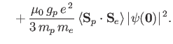
 . The associated magnetic field takes the form [49]
![$\displaystyle {\bf B}=\nabla\times {\bf A} =\frac{\mu_0}{4\pi}\left[ \frac{3\,({\bf M}\cdot{\bf e}_r)\,{\bf e}_r-{\bf M}}{r^{\,3}}\right],$](img2072.png) |
(7.143) |
where
 . Suppose that
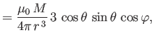
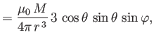
 . The
Cartesian components of
. The
Cartesian components of  are thus
where ( ,
,  ,
,  ) are conventional spherical coordinates. It
is easily demonstrated that
) are conventional spherical coordinates. It
is easily demonstrated that
 |
(7.147) |
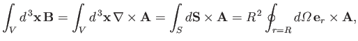
where  is a spherical volume of radius
  , centered on the origin. However,
we can also write [67]
, centered on the origin. However,
we can also write [67]
 |
(7.148) |
where  is the bounding surface of volume
, and
is the bounding surface of volume
, and
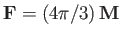
 an element of solid angle. According to Equation (7.145),
Let
, and
 .
It follows that
.
It follows that
which implies that
 .
Hence, we obtain
.
Hence, we obtain
 |
(7.153) |
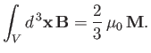
However, the previous expression is inconsistent with Equations (7.147)-(7.149). Note that
the right-hand side of Equation (7.156) is independent of the radius,
, of the integration volume
.
Consequently, we can take the limit
 without changing the value of
 .
We deduce that the non-zero contribution to this integral originates from the origin. Hence, we can
reconcile the previously mentioned inconsistency by modifying Equation (7.146) to read
.
We deduce that the non-zero contribution to this integral originates from the origin. Hence, we can
reconcile the previously mentioned inconsistency by modifying Equation (7.146) to read
![$\displaystyle {\bf B} =\frac{\mu_0}{4\pi}\left[ \frac{3\,({\bf M}\cdot{\bf e}_r...
...-{\bf M}}{r^{\,3}}\right] + \frac{2\,\mu_0}{3}\,\delta^{\,3}({\bf x})\,{\bf M}.$](img2099.png) |
(7.154) |
Here,
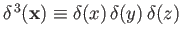 is a three-dimensional Dirac delta function. This function has the property that
 |
(7.155) |
where
 is a general function that is well-behaved in the vicinity of
 (which is
assumed to lie in the volume
) [92].
(which is
assumed to lie in the volume
) [92].
According to the previous formula, the proton's magnetic moment,
, generates a
magnetic field of the form
![$\displaystyle {\bf B} = \frac{\mu_0}{4\pi\,r^{\,3}}\,\left[3\,(\mbox{\boldmath$...
...p\right] + \frac{2\,\mu_0}{3}\,\delta^{\,3}({\bf x})\,\mbox{\boldmath$\mu$}_p\,$](img2104.png) |
(7.156) |
where  measures position relative to the proton. Now, the Hamiltonian of the electron in the magnetic
field generated by the proton is simply [49]
measures position relative to the proton. Now, the Hamiltonian of the electron in the magnetic
field generated by the proton is simply [49]
where
 |
(7.158) |
Here,
 is the electron magnetic moment [see Equation (7.98)], and
  the electron spin. Thus, the
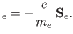
perturbing Hamiltonian is written
the electron spin. Thus, the
perturbing Hamiltonian is written
 |
(7.159) |
Note that, because we have neglected coupling between the proton
spin and the magnetic field generated by the electron's orbital motion,
the previous expression is only valid for  states.
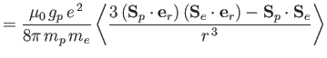
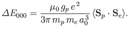
According to standard first-order perturbation theory, the energy-shift induced
by spin-spin coupling between the proton and the electron is the expectation
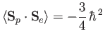
value of the perturbing Hamiltonian. Hence,
In the final term on the right-hand side, the expectation value is taken over the overall spin state.
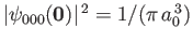
For the ground state of hydrogen, which is spherically symmetric,
the first term in the previous expression vanishes by symmetry.
Moreover, it is easily demonstrated that
 . Thus, we obtain
 |
(7.161) |
Let
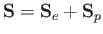 |
(7.162) |
be the total spin. We can show that
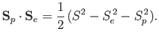 |
(7.163) |
Thus, the simultaneous eigenstates of the perturbing Hamiltonian
and the main Hamiltonian are the simultaneous eigenstates of  ,
,
 , and
, and  . (The use of simultaneous eigenstates of the perturbing and main Hamiltonian
avoids the possibility of singular terms arising in the perturbation expansion to second order--see Section 7.5.) However, both the proton and
the electron are spin one-half particles. According to Section 6.4,
when two spin one-half particles are combined (in the absence of orbital
angular momentum) the resulting state has either spin 1 or spin 0.
In fact, there are three spin 1 states, known as triplet states, and a single
spin 0 state, known as the singlet state. For all states,
the eigenvalues of
and
are
. (The use of simultaneous eigenstates of the perturbing and main Hamiltonian
avoids the possibility of singular terms arising in the perturbation expansion to second order--see Section 7.5.) However, both the proton and
the electron are spin one-half particles. According to Section 6.4,
when two spin one-half particles are combined (in the absence of orbital
angular momentum) the resulting state has either spin 1 or spin 0.
In fact, there are three spin 1 states, known as triplet states, and a single
spin 0 state, known as the singlet state. For all states,
the eigenvalues of
and
are
 .
The eigenvalue of
is 0 for the singlet state, and
.
The eigenvalue of
is 0 for the singlet state, and
 for the triplet states. Hence,
 |
(7.164) |
for the singlet state, and
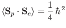 |
(7.165) |
for the triplet states.
It follows, from the previous analysis, that proton-electron spin-spin coupling breaks
the degeneracy of the two
 states of the hydrogen atom, lifting the
energy of the triplet configuration, and lowering that of the singlet.
This splitting is known as hyperfine structure.
The net energy difference between the singlet and the triplet states
is
states of the hydrogen atom, lifting the
energy of the triplet configuration, and lowering that of the singlet.
This splitting is known as hyperfine structure.
The net energy difference between the singlet and the triplet states
is
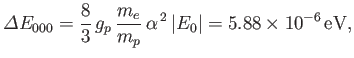 |
(7.166) |
where
 is the (magnitude of the) ground-state energy, and
 the
fine structure constant.
Note that the hyperfine energy-shift is much smaller, by a factor
, than
a typical fine structure energy-shift. (See Exercise 14.)
If we convert the previous energy into a wavelength (using
the
fine structure constant.
Note that the hyperfine energy-shift is much smaller, by a factor
, than
a typical fine structure energy-shift. (See Exercise 14.)
If we convert the previous energy into a wavelength (using
 ) then we obtain
 |
(7.167) |
This is the wavelength of the radiation emitted by a hydrogen atom
that is collisionally excited from the singlet to the triplet
state, and then decays back to the lower energy singlet state.
The 21cm line is famous in radio astronomy because it was used to
map out the spiral structure of our galaxy in the 1950's [114].
Next: Exercises
Up: Time-Independent Perturbation Theory
Previous: Zeeman Effect
Richard Fitzpatrick
2016-01-22

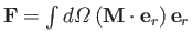
![$\displaystyle =\frac{\mu_0}{4\pi} \oint d{\mit\Omega}\,{\bf e}_r\times ({\bf M}...
...u_0}{4\pi} \oint d{\mit\Omega} \,[{\bf M} - ({\bf M}\cdot{\bf e}_r)\,{\bf e}_r]$](img2086.png)