Next: Zeeman Effect
Up: Time-Independent Perturbation Theory
Previous: Linear Stark Effect
Fine Structure
Let us now consider the energy levels of hydrogen-like atoms (i.e., alkali
metal atoms) in more detail. The outermost electron moves in a spherically
symmetric potential,  , generated by the nuclear charge and the charges of the
other electrons (which occupy spherically symmetric closed shells). Thus, according to
Section 4.5, we can label the energy eigenstates of the outermost electron using the
conventional quantum numbers
, generated by the nuclear charge and the charges of the
other electrons (which occupy spherically symmetric closed shells). Thus, according to
Section 4.5, we can label the energy eigenstates of the outermost electron using the
conventional quantum numbers  ,
,  , and
, and  . However, the
shielding effect of the inner electrons causes
to depart from
the pure Coulomb form. This splits the degeneracy of states characterized by the
same value of
, but different values of
. In fact, higher
states
have higher energies.
. However, the
shielding effect of the inner electrons causes
to depart from
the pure Coulomb form. This splits the degeneracy of states characterized by the
same value of
, but different values of
. In fact, higher
states
have higher energies.
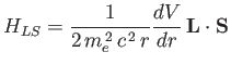
Let us examine a phenomenon known as fine structure, which caused by the
interaction between the spin and orbital angular momenta of the outermost
electron. This electron experiences an electric field [49]
 |
(7.95) |
However, a non-relativistic charge moving in an electric field also experiences an effective
magnetic field [49]
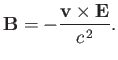 |
(7.96) |
Now, an electron possesses a spin magnetic moment
 |
(7.97) |
[See Equation (5.47).]
We, therefore, expect a contribution to the Hamiltonian of
the form [49]
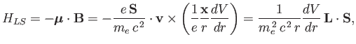 |
(7.98) |
where
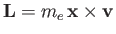 is the orbital angular momentum.
This phenomenon is known as spin-orbit coupling.
Actually, when the previous expression is compared to the experimentally observed spin-orbit interaction,
it is found to be too large by a factor of two. There is a classical explanation
for this discrepancy which involves a precession of the electron spin--the so-called Thomas precession--caused by the relativistic time dilation between the orbiting electron and the atomic nucleus [109]. The
quantum mechanical explanation requires a relativistically covariant
treatment of the electron dynamics [32,9].
is the orbital angular momentum.
This phenomenon is known as spin-orbit coupling.
Actually, when the previous expression is compared to the experimentally observed spin-orbit interaction,
it is found to be too large by a factor of two. There is a classical explanation
for this discrepancy which involves a precession of the electron spin--the so-called Thomas precession--caused by the relativistic time dilation between the orbiting electron and the atomic nucleus [109]. The
quantum mechanical explanation requires a relativistically covariant
treatment of the electron dynamics [32,9].
Let us now apply perturbation theory to a hydrogen-like atom, using
 |
(7.99) |
as the perturbation (noting that  takes one half of the value given previously), and
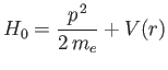 |
(7.100) |
as the unperturbed Hamiltonian. We have two choices for the energy
eigenstates of  . We can adopt the simultaneous eigenstates of
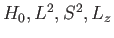 and
and  , or the simultaneous eigenstates of
 and
and  , where
 is
the total angular momentum. Although the departure of
from a pure
is
the total angular momentum. Although the departure of
from a pure
 form splits the degeneracy of same
, different
, states,
those states characterized by the same values of
and
, but different
values of
form splits the degeneracy of same
, different
, states,
those states characterized by the same values of
and
, but different
values of  , are still degenerate.
(Here,
, are still degenerate.
(Here,  and
and  are the quantum numbers
corresponding to
are the quantum numbers
corresponding to  and
, respectively.)
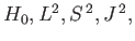
Moreover, with the addition of spin
degrees of freedom, each state is doubly degenerate because of the two possible
orientations of the electron spin (i.e.,
and
, respectively.)
Moreover, with the addition of spin
degrees of freedom, each state is doubly degenerate because of the two possible
orientations of the electron spin (i.e.,
 ). Thus, we are still
dealing with a
highly degenerate system. However, we know, from Section 7.5, that there is no
danger of singular terms appearing to second order in the perturbation expansion if the
degenerate eigenstates of the unperturbed Hamiltonian (and the set of commuting operators needed to
uniquely label the degenerate eigenstates) are also eigenstates of the perturbing Hamiltonian. Now, the perturbing Hamiltonian,
, is proportional to
). Thus, we are still
dealing with a
highly degenerate system. However, we know, from Section 7.5, that there is no
danger of singular terms appearing to second order in the perturbation expansion if the
degenerate eigenstates of the unperturbed Hamiltonian (and the set of commuting operators needed to
uniquely label the degenerate eigenstates) are also eigenstates of the perturbing Hamiltonian. Now, the perturbing Hamiltonian,
, is proportional to
 , where
 |
(7.101) |
It is fairly obvious
that the first group of operators (
and
)
does not commute with
, whereas the second group
(
and
) does. In fact,
is just a combination of operators appearing in the second group. Thus, it is
advantageous to work in terms of the eigenstates of the second group of
operators, rather than those of the first group (because the former eigenstates are also eigenstates
of the perturbing Hamiltonian).
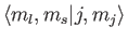
We now need to find the simultaneous eigenstates of
and
.
This is equivalent to finding the eigenstates of the total angular momentum
resulting from the addition of two angular momenta:  , and
, and
 .
According to Equation (6.26), the allowed values of the total angular
momentum are
.
According to Equation (6.26), the allowed values of the total angular
momentum are  and
and  . We can write
Here, the kets on the left-hand side are
 kets, whereas
those on the right-hand side are
kets, whereas
those on the right-hand side are
 kets
(the
kets
(the  labels have been dropped, for the sake of clarity). We have made use
of the fact that the Clebsch-Gordon coefficients are automatically
zero unless
labels have been dropped, for the sake of clarity). We have made use
of the fact that the Clebsch-Gordon coefficients are automatically
zero unless
 . (See Section 6.3.) We have also made use of the fact that
both the
and
kets are orthonormal. We now need to determine
. (See Section 6.3.) We have also made use of the fact that
both the
and
kets are orthonormal. We now need to determine
 |
(7.104) |
where the Clebsch-Gordon coefficient is written in
 form.
form.
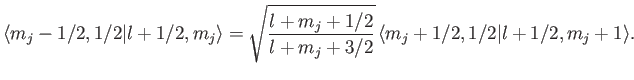
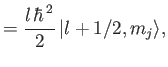
Let us now employ the recursion relation for Clebsch-Gordon coefficients, Equation (6.32),
with
,  ,
,
,
,
 , and
, and  , choosing the lower sign.
We obtain
, choosing the lower sign.
We obtain
which reduces to
 |
(7.105) |
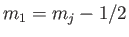
We can use this formula to successively increase the value of
. For
instance,
This procedure can be continued until
attains its maximum possible value,
. Thus,
 |
(7.106) |
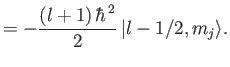
Consider the situation in which
and  both take their maximum values,
and
both take their maximum values,
and  , respectively. The corresponding value of
is
, respectively. The corresponding value of
is
 . This value is possible when
, but not when
.
Thus, the
ket
. This value is possible when
, but not when
.
Thus, the
ket
 must be equal to
the
ket
must be equal to
the
ket
 , up to an arbitrary phase-factor.
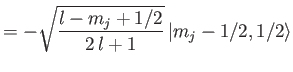
By convention, this factor is taken to be unity, giving
, up to an arbitrary phase-factor.
By convention, this factor is taken to be unity, giving
 |
(7.107) |
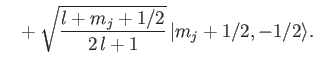
It follows from Equation (7.109) that
 |
(7.108) |
Hence,
 |
(7.109) |
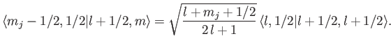
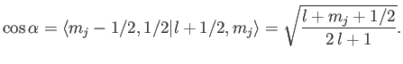
We now need to determine the sign of
 . A careful examination
of the recursion relation, Equation (6.32), shows that the plus sign is
appropriate. Thus,
. A careful examination
of the recursion relation, Equation (6.32), shows that the plus sign is
appropriate. Thus,
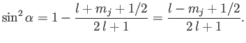
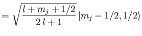
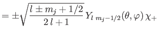
It is convenient to define so-called spin-angular functions using the
Pauli two-component formalism:
(See Section 5.7.)
These functions are eigenfunctions of the total angular momentum for spin
one-half particles, just as the spherical harmonics are eigenfunctions
of the orbital angular momentum. A general spinor-wavefunction for an energy
eigenstate in a hydrogen-like atom is written
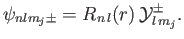 |
(7.113) |
The radial part of the wavefunction,
 , depends on the principal
quantum number
, and the azimuthal quantum number
. The wavefunction
is also
labeled by
, which is the quantum number associated with
.
For a given choice of
, the quantum number
, depends on the principal
quantum number
, and the azimuthal quantum number
. The wavefunction
is also
labeled by
, which is the quantum number associated with
.
For a given choice of
, the quantum number  (i.e., the quantum number associated with
  ) can take the values
 . (However,
  for the special case
  .)
.)
The
 kets are eigenstates of
,
according to Equation (7.102).
Thus,
kets are eigenstates of
,
according to Equation (7.102).
Thus,
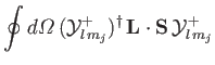
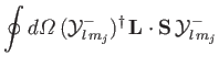
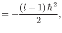
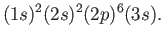
![$\displaystyle {\bf L} \cdot{\bf S}\, \vert j=l\pm 1/2,m_j\rangle = \frac{\hbar^{\,2}}{2} \left[ j\,(j+1) - l\,(l+1) - 3/4\right]\vert j,m_j\rangle,$](img1984.png) |
(7.114) |
giving
It follows that
where the integrals are over all solid angle,
 .
.
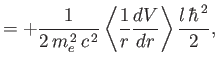
Let us now apply degenerate perturbation theory to evaluate the
energy-shift of a state whose spinor-wavefunction is
 caused by the spin-orbit Hamiltonian,
. To first order, the energy-shift is given by
caused by the spin-orbit Hamiltonian,
. To first order, the energy-shift is given by
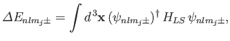 |
(7.119) |
where the integral is over all space,
 . Equations (7.100), (7.116), and (7.120)-(7.121) yield
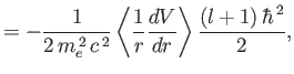
where
 |
(7.122) |
Incidentally, for the special case of an
state,
 , and
there is no state with
, so Equation (7.124) is redundant. Thus, it is clear that
, and
there is no state with
, so Equation (7.124) is redundant. Thus, it is clear that
 for an
state, which is not surprising, given that such a state possesses zero
orbital angular momentum (i.e., it is characterized by
for an
state, which is not surprising, given that such a state possesses zero
orbital angular momentum (i.e., it is characterized by
 .)
.)
Let us now apply the previous result to the case of a sodium atom.
In chemist's notation [53], the ground state is written
 |
(7.123) |
[Here,  implies that there are two electrons in the
  state, et cetera.]
The inner ten electrons effectively form a spherically symmetric electron
cloud. We are interested in the excitation of the eleventh electron
from
state, et cetera.]
The inner ten electrons effectively form a spherically symmetric electron
cloud. We are interested in the excitation of the eleventh electron
from  to some higher energy state. The closest (in energy) unoccupied
state is
to some higher energy state. The closest (in energy) unoccupied
state is  . This state has a higher energy than
due to the deviations
of the potential from the pure Coulomb form. In the absence of spin-orbit
interaction, there are six degenerate
states. The spin-orbit
interaction breaks the degeneracy of these states. The modified states are
labeled
. This state has a higher energy than
due to the deviations
of the potential from the pure Coulomb form. In the absence of spin-orbit
interaction, there are six degenerate
states. The spin-orbit
interaction breaks the degeneracy of these states. The modified states are
labeled
 and
and
 , where the subscript refers to the
value of
. The four
states lie at a slightly higher
energy level than the two
states,
because the radial integral (7.125) is positive. (See Exercise 14.) The splitting of
the
, where the subscript refers to the
value of
. The four
states lie at a slightly higher
energy level than the two
states,
because the radial integral (7.125) is positive. (See Exercise 14.) The splitting of
the  energy levels of the sodium atom can be observed
using a spectroscope (which measures the frequency of spectral lines caused by transitions
between quantum states of different energy--this frequency is, of course,
energy levels of the sodium atom can be observed
using a spectroscope (which measures the frequency of spectral lines caused by transitions
between quantum states of different energy--this frequency is, of course,
 --see Section 8.9).
The well-known sodium D-line is associated with transitions between
the
and
states. The fact that there are two slightly different
energy levels (note that spin-orbit coupling does not split
the
energy levels) means that the sodium D-line actually consists
of two very closely spaced (in frequency) spectroscopic lines. It is easily
demonstrated that the ratio of the typical spacing of
Paschen lines (i.e., spectral lines associated with transitions to the 3s state [61]) to the splitting
brought about by spin-orbit interaction is about
--see Section 8.9).
The well-known sodium D-line is associated with transitions between
the
and
states. The fact that there are two slightly different
energy levels (note that spin-orbit coupling does not split
the
energy levels) means that the sodium D-line actually consists
of two very closely spaced (in frequency) spectroscopic lines. It is easily
demonstrated that the ratio of the typical spacing of
Paschen lines (i.e., spectral lines associated with transitions to the 3s state [61]) to the splitting
brought about by spin-orbit interaction is about
 ,
where
,
where
 is the fine structure constant. (See Exercise 14.) Actually, Equations (7.123)-(7.124) are not
entirely correct, because we have neglected an effect (namely, the
relativistic mass increase of the electron) that is the same
order of magnitude as spin-orbit coupling. (See Exercises 11-14.)
is the fine structure constant. (See Exercise 14.) Actually, Equations (7.123)-(7.124) are not
entirely correct, because we have neglected an effect (namely, the
relativistic mass increase of the electron) that is the same
order of magnitude as spin-orbit coupling. (See Exercises 11-14.)
Next: Zeeman Effect
Up: Time-Independent Perturbation Theory
Previous: Linear Stark Effect
Richard Fitzpatrick
2016-01-22
![\begin{multline}[(l+1/2)\,(l+3/2)-m_j\,(m_j+1)]^{1/2} \,\langle m_j-1/2, 1/2\ver...
...(m_j+1/2)]^{1/2}\, \langle m_j+1/2, 1/2\vert l+1/2, m_j+1\rangle,
\end{multline}](img1960.png)
![\begin{multline}
\langle m_j-1/2, 1/2\vert l+1/2, m_j\rangle\\ [0.5ex] =\sqrt{\f...
.../2}{l+m_j+5/2}} \, \langle m_j+3/2, 1/2\vert l+1/2, m_j+2\rangle.
\end{multline}](img1962.png)

![$\displaystyle = \frac{1}{\sqrt{2\,l+1}}\left(\begin{array}{c} \pm \sqrt{l\pm m_...
...] \sqrt{l\mp m_j+1/2}\,\,Y_{l\,\,m_j+1/2}(\theta, \varphi) \end{array} \right).$](img1978.png)