


Next: Gauge Transformations in Electromagnetism
Up: Quantum Dynamics
Previous: Schrödinger Wave Equation
Charged Particle Motion in Electromagnetic Fields
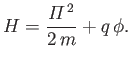
The classical Hamiltonian for a particle of mass  and charge
  moving under the influence of
electromagnetic fields is [55]
moving under the influence of
electromagnetic fields is [55]
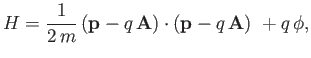 |
(3.71) |
where
 and
and
 are the vector and scalar potentials, respectively [49]. These potentials are related to the familiar electric and magnetic field-strengths,
 and
and
 , respectively, via [49]
Let us assume that expression (3.71) is also the correct quantum mechanical Hamiltonian for
a charged particle moving in electromagnetic fields. Obviously, in quantum mechanics, we must treat  ,
,  , and
, and  as operators that do not necessarily commute.
The Heisenberg equations of motion for the components of  are
are
![$\displaystyle \frac{dx_i}{dt} =\frac{[x_i, H]}{{\rm i}\,\hbar}.$](img730.png) |
(3.74) |
However,
![$\displaystyle [x_i, H] = {\rm i}\,\hbar\,\frac{\partial H}{\partial p_i} = \frac{{\rm i}\,\hbar}{m}\,(p_i-q\,A_i),$](img731.png) |
(3.75) |
where use has been made of Equations (3.33) and (3.71).
It follows that
where
  |
(3.77) |
Here,
 is referred to as the mechanical momentum, whereas
is termed the canonical
momentum.
is referred to as the mechanical momentum, whereas
is termed the canonical
momentum.
It is easily seen that
![$\displaystyle [{\mit\Pi}_i, {\mit\Pi}_j] = q\,[p_j, A_i] -q\,[p_i, A_j].$](img737.png) |
(3.78) |
However,
![$\displaystyle [p_j, A_i] = -{\rm i}\,\hbar\,\frac{\partial A_i}{\partial x_j},$](img738.png) |
(3.79) |
where we have employed Equation (3.34).
Thus, we obtain
![$\displaystyle [{\mit\Pi}_i, {\mit\Pi}_j] = {\rm i}\,\hbar\,q\left(\frac{\partia...
...rac{\partial A_i}{\partial x_j}\right)= {\rm i}\,\hbar\,q\,\epsilon_{ijk}\,B_k,$](img739.png) |
(3.80) |
because [from Equation (3.73)]
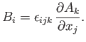 |
(3.81) |
Here,
 is the totally antisymmetric tensor (that is,
 if
if  ,
,  ,
,  is a cyclic permutation of
  ,
,  ,
,  ;
;
 if
,
,
is an anti-cyclic permutation
of
,
,
; and
if
,
,
is an anti-cyclic permutation
of
,
,
; and
 otherwise), and we have used the standard result
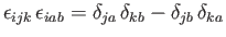 , as well as the
Einstein summation convention (that repeated indices are implicitly summed from
to
) [92].
, as well as the
Einstein summation convention (that repeated indices are implicitly summed from
to
) [92].
We can write the Hamiltonian (3.71) in the form
 |
(3.82) |
The Heisenberg equation of motions for the components of
are
![$\displaystyle \frac{d{\mit\Pi}_i}{dt}=\frac{[{\mit\Pi}_i, H]}{{\rm i}\,\hbar} + \frac{\partial {\mit\Pi}_i}{\partial t}.$](img750.png) |
(3.83) |
Here, we have taken into account the fact that
 depends explicitly on time through its dependence on
 .
However,
.
However,
![$\displaystyle [{\mit\Pi}_i, {\mit\Pi}^{\,2}] = {\mit\Pi}_j\,[{\mit\Pi}_i, {\mit...
...\left(\epsilon_{ijk}\,{\mit\Pi}_j\,B_k-\epsilon_{ijk}\,B_j\,{\mit\Pi}_k\right),$](img753.png) |
(3.84) |
where use has been made of Equation (3.80).
Moreover,
where we have employed Equation (3.33).
The previous five equations yield
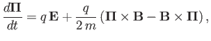 |
(3.87) |
which can be combined with Equation (3.76) to give
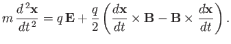 |
(3.88) |
This equation of motion is a generalization of the Ehrenfest theorem that takes electromagnetic fields
into account. The fact that Equation (3.88) is analogous in form to the
corresponding classical equation of motion (given that
 and
and  commute in classical mechanics)
justifies our earlier assumption that Equation (3.71) is the correct quantum mechanical Hamiltonian for
a charged particle moving in electromagnetic fields.
commute in classical mechanics)
justifies our earlier assumption that Equation (3.71) is the correct quantum mechanical Hamiltonian for
a charged particle moving in electromagnetic fields.
Next: Gauge Transformations in Electromagnetism
Up: Quantum Dynamics
Previous: Schrödinger Wave Equation
Richard Fitzpatrick
2016-01-22

![$\displaystyle = [p_i, \phi] = -{\rm i}\,\hbar\,\frac{\partial\phi}{\partial x_i},$](img757.png)
