Next: Born Approximation
Up: Scattering Theory
Previous: Introduction
Consider time-independent scattering theory, for which the Hamiltonian
of the system is written
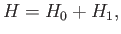 |
(10.1) |
where
 |
(10.2) |
is the Hamiltonian of a free particle of mass  ,
and
,
and  represents the non-time-varying source of the scattering. Let
 be an energy eigenket of
  ,
,
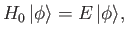 |
(10.3) |
whose wavefunction is
 . This wavefunction is assumed to be a plane wave.
Schrödinger's equation for the scattering problem is
. This wavefunction is assumed to be a plane wave.
Schrödinger's equation for the scattering problem is
 |
(10.4) |
where
 is an energy eigenstate of the total Hamiltonian
whose wavefunction is
is an energy eigenstate of the total Hamiltonian
whose wavefunction is
 .
In general, both
and
.
In general, both
and  have continuous energy
spectra: that is, their energy eigenstates are unbound.
We require a solution of Equation (10.4) that satisfies the
boundary condition
have continuous energy
spectra: that is, their energy eigenstates are unbound.
We require a solution of Equation (10.4) that satisfies the
boundary condition
 as
as
 . Here,
is a solution of the free-particle
Schrödinger equation, (10.3), that corresponds to the same energy eigenvalue as
.
. Here,
is a solution of the free-particle
Schrödinger equation, (10.3), that corresponds to the same energy eigenvalue as
.
Adopting the Schrödinger representation (see Section 2.4), we can write the scattering
equation, (10.4), in the form
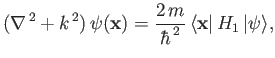 |
(10.5) |
where
 |
(10.6) |
(See Exercise 1.)
Equation (10.5) is known as the Helmholtz equation, and can be inverted
using standard Green's function techniques [49]. Thus,
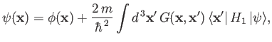 |
(10.7) |
where
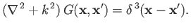 |
(10.8) |
(See Exercise 2.)
Here,
 is a three-dimensional Dirac delta function.
Note that the solution (10.7) satisfies the previously mentioned constraint
as
.
As is well known, the Green's function for the Helmholtz equation is
given by
is a three-dimensional Dirac delta function.
Note that the solution (10.7) satisfies the previously mentioned constraint
as
.
As is well known, the Green's function for the Helmholtz equation is
given by
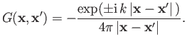 |
(10.9) |
(See Exercise 3.)
Thus, Equation (10.7) becomes
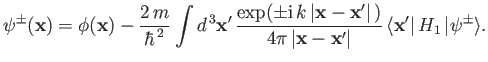 |
(10.10) |
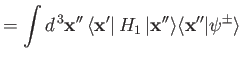
Let us suppose that the scattering Hamiltonian,
, is a function only
of the position operators. This implies that
 |
(10.11) |
We can write
where use has been made of the standard completeness relation
 . (See Section 1.15.)
Thus, the integral equation (10.10) simplifies to give
. (See Section 1.15.)
Thus, the integral equation (10.10) simplifies to give
 |
(10.13) |
Suppose that the initial state,
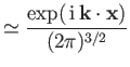
, possesses a plane-wave wavefunction with wavevector  (i.e., it corresponds to a stream of particles of
definite momentum
(i.e., it corresponds to a stream of particles of
definite momentum
 ). The ket corresponding to
this state is denoted
). The ket corresponding to
this state is denoted
 . Thus,
 |
(10.14) |
The preceding wavefunction is conveniently normalized such that
![$\displaystyle \langle {\bf k}\vert{\bf k}'\rangle =\int d^{\,3} {\bf x}\, \lang...
...f x}\cdot({\bf k} -{\bf k}')]} {(2\pi )^3} = \delta^{\,3} ({\bf k} - {\bf k'}).$](img3433.png) |
(10.15) |
(See Section 2.6 and Exercise 4.)
Suppose that the scattering potential,
 , is non-zero only in some
relatively localized region centered on the origin (
, is non-zero only in some
relatively localized region centered on the origin (
 ).
Let us calculate the total wavefunction,
).
Let us calculate the total wavefunction,
 , far from
the scattering region. In other words, let us adopt the ordering
, far from
the scattering region. In other words, let us adopt the ordering
 , where
 and
and
 . It is easily demonstrated that
 |
(10.16) |
to first order in  , where
 is a unit vector that is directed from the scattering region to the
observation point. Let us define
is a unit vector that is directed from the scattering region to the
observation point. Let us define
 |
(10.17) |
Clearly,  is the wavevector for particles that possess the
same energy as the incoming particles (i.e.,
is the wavevector for particles that possess the
same energy as the incoming particles (i.e.,  ), but propagate
from the scattering region to the observation point. Note that
), but propagate
from the scattering region to the observation point. Note that
 |
(10.18) |
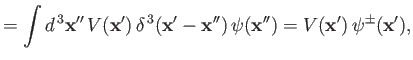
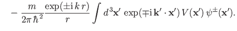
In the large- limit, Equations (10.13) and (10.14) reduce to
The first term on the right-hand side of the previous equation is the incident wave. The second term
represents a spherical wave centered on the scattering region. The
plus sign (on  ) corresponds to a wave propagating away from the
scattering region, whereas the minus sign corresponds to a
wave propagating toward the scattering region. (See Exercise 5.) It is obvious that
the former represents the physical solution.
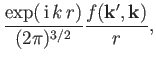
Thus, the wavefunction far from the scattering region can be
written
) corresponds to a wave propagating away from the
scattering region, whereas the minus sign corresponds to a
wave propagating toward the scattering region. (See Exercise 5.) It is obvious that
the former represents the physical solution.
Thus, the wavefunction far from the scattering region can be
written
![$\displaystyle \psi({\bf x}) = \frac{1}{(2\pi)^{3/2}} \left[\exp(\,{\rm i}\,{\bf k}\cdot{\bf x}) + \frac{\exp(\,{\rm i}\,k\,r)}{r} f({\bf k}', {\bf k}) \right],$](img3448.png) |
(10.20) |
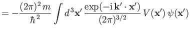
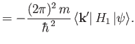
where
[See Equations (10.11) and (10.14).]
Let us define the differential scattering cross-section,
 , as
the number of particles per unit time scattered into an element of
solid angle
, as
the number of particles per unit time scattered into an element of
solid angle
 , divided by the incident particle flux.
Recall, from Chapter 3, that the probability current
(which is proportional to the particle flux) associated with a
wavefunction
, divided by the incident particle flux.
Recall, from Chapter 3, that the probability current
(which is proportional to the particle flux) associated with a
wavefunction  is
is
 |
(10.22) |
Thus, the particle flux associated with the incident wavefunction,
 |
(10.23) |
is proportional to
 |
(10.24) |
Likewise, the particle flux associated with the scattered wavefunction,
 |
(10.25) |
is proportional to
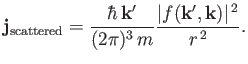 |
(10.26) |
Now, by definition,
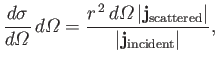 |
(10.27) |
giving
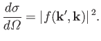 |
(10.28) |
Thus,
 is the differential cross-section for particles with incident momentum
 to be scattered
into states whose momentum vectors are directed in a range of solid angles
about
to be scattered
into states whose momentum vectors are directed in a range of solid angles
about
 . Note that the scattered particles possess
the same energy as the incoming particles (i.e.,
). This is always
the case for scattering Hamiltonians of the form specified in Equation (10.11).
. Note that the scattered particles possess
the same energy as the incoming particles (i.e.,
). This is always
the case for scattering Hamiltonians of the form specified in Equation (10.11).
Next: Born Approximation
Up: Scattering Theory
Previous: Introduction
Richard Fitzpatrick
2016-01-22