Suppose that we have found an inertial frame of reference. Let us
set up a Cartesian coordinate system in this frame. The motion
of a point object can now be specified by giving its position vector,
![]() ,
with respect to the origin of the coordinate system, as a function of time,
,
with respect to the origin of the coordinate system, as a function of time, ![]() .
Consider a second frame of reference moving with some
constant velocity
.
Consider a second frame of reference moving with some
constant velocity
![]() with respect to the first frame. Without loss of generality,
we can suppose that the Cartesian axes in the second frame are parallel
to the corresponding axes in the first frame, that
with respect to the first frame. Without loss of generality,
we can suppose that the Cartesian axes in the second frame are parallel
to the corresponding axes in the first frame, that
![]() ,
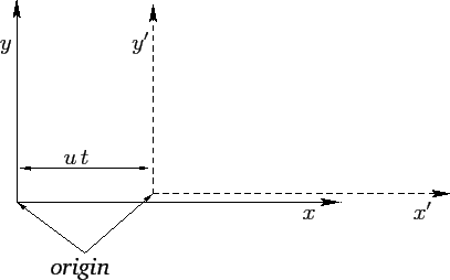
and, finally, that the origins of the two frames instantaneously coincide at
,
and, finally, that the origins of the two frames instantaneously coincide at ![]() --see Figure 1. Suppose that the position vector
of our point object is
--see Figure 1. Suppose that the position vector
of our point object is
![]() in the second frame of reference.
It is evident, from Figure 1, that at any given time,
in the second frame of reference.
It is evident, from Figure 1, that at any given time, ![]() , the coordinates of the
object in the two reference frames satisfy
, the coordinates of the
object in the two reference frames satisfy
By definition, the instantaneous velocity of the object in our first reference frame is given by
![]() , with an analogous
expression for the velocity,
, with an analogous
expression for the velocity, ![]() , in the second frame.
It follows from differentiation of Equations (1)-(3) with respect to time that the velocity components in the two frames satisfy
, in the second frame.
It follows from differentiation of Equations (1)-(3) with respect to time that the velocity components in the two frames satisfy
Finally, by definition, the instantaneous acceleration of the object in our first reference frame is given by
![]() , with an analogous
expression for the acceleration,
, with an analogous
expression for the acceleration, ![]() , in the second frame.
It follows from differentiation of Equations (4)-(6) with respect to time that the acceleration
components in the two frames satisfy
, in the second frame.
It follows from differentiation of Equations (4)-(6) with respect to time that the acceleration
components in the two frames satisfy
| (8) | |||
| (9) | |||
| (10) |
According to Equations (7) and (11), if an
object is moving in a straight-line with constant speed in our original
inertial frame (i.e., if
![]() ) then it also
moves in a (different) straight-line with (a different) constant speed
in the second frame of reference (i.e.,
) then it also
moves in a (different) straight-line with (a different) constant speed
in the second frame of reference (i.e.,
![]() ). Hence,
we conclude that the second frame of reference is also an inertial frame.
). Hence,
we conclude that the second frame of reference is also an inertial frame.
A simple extension of the above argument allows us to conclude that there are an infinite number of different inertial frames moving with constant velocities with respect to one another. Newton through that one of these inertial frames was special, and defined an absolute standard of rest: i.e., a static object in this frame was in a state of absolute rest. However, Einstein showed that this is not the case. In fact, there is no absolute standard of rest: i.e., all motion is relative--hence, the name ``relativity'' for Einstein's theory. Consequently, one inertial frame is just as good as another as far as Newtonian dynamics is concerned.
But, what happens if the second frame of reference accelerates with
respect to the first? In this case, it is not hard to see that Equation (11)
generalizes to
| (12) |
A simple extension of the above argument allows us to conclude that any frame of reference which accelerates with respect to a given inertial frame is not itself an inertial frame.
For most practical purposes, when studying the motions of objects close to the Earth's surface, a reference frame which is fixed with respect to this surface is approximately inertial. However, if the trajectory of a projectile within such a frame is measured to high precision then it will be found to deviate slightly from the predictions of Newtonian dynamics--see Chapter 7. This deviation is due to the fact that the Earth is rotating, and its surface is therefore accelerating towards its axis of rotation. When studying the motions of objects in orbit around the Earth, a reference frame whose origin is the center of the Earth, and whose coordinate axes are fixed with respect to distant stars, is approximately inertial. However, if such orbits are measured to extremely high precision then they will again be found to deviate very slightly from the predictions of Newtonian dynamics. In this case, the deviation is due to the Earth's orbital motion about the Sun. When studying the orbits of the planets in the Solar System, a reference frame whose origin is the center of the Sun, and whose coordinate axes are fixed with respect to distant stars, is approximately inertial. In this case, any deviations of the orbits from the predictions of Newtonian dynamics due to the orbital motion of the Sun about the galactic center are far too small to be measurable. It should be noted that it is impossible to identify an absolute inertial frame--the best approximation to such a frame would be one in which the cosmic microwave background appears to be (approximately) isotropic. However, for a given dynamical problem, it is always possible to identify an approximate inertial frame. Furthermore, any deviations of such a frame from a true inertial frame can be incorporated into the framework of Newtonian dynamics via the introduction of so-called fictitious forces--see Chapter 7.