Centrifugal Acceleration

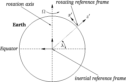
Let our non-rotating inertial frame be one whose origin lies at the center of the Earth, and let our rotating frame be one whose origin is fixed with respect to some point, of latitude $\lambda$, on the Earth's surface--see Figure 24. The latter reference frame thus rotates with respect to the former (about an axis passing through the Earth's center) with an angular velocity vector, $\mbox{\boldmath$\Omega$}$, which points from the center of the Earth toward its north pole, and is of magnitude

$${\mit\Omega} = \frac{2\pi}{24\,\,{\rm hrs}}=7.27\times 10^{-5}\,{\rm rad./s}.$$ (415)

Figure 24: Inertial and non-inertial reference frames.

Consider an object which appears stationary in our rotating reference frame: i.e., an object which is stationary with respect to the Earth's surface. According to Equation (414), the object's apparent equation of motion in the rotating frame takes the form

$$m\,{\bf a}' = {\bf f} - m\,\mbox{\boldmath$\Omega$}\times(\mbox{\boldmath$\Omega$}\times{\bf r}).$$ (416)

Let the non-fictitious force acting on our object be the force of gravity, ${\bf f}= m\,{\bf g}$. Here, the local gravitational acceleration, ${\bf g}$, points directly toward the center of the Earth. It follows, from the above, that the apparent gravitational acceleration in the rotating frame is written

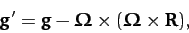$${\bf g}' = {\bf g} - \mbox{\boldmath$\Omega$}\times(\mbox{\boldmath$\Omega$}\times{\bf R}),$$ (417)

where ${\bf R}$ is the displacement vector of the origin of the rotating frame (which lies on the Earth's surface) with respect to the center of the Earth. Here, we are assuming that our object is situated relatively close to the Earth's surface (i.e., ${\bf r}\simeq {\bf R}$).

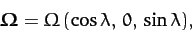
It can be seen, from Equation (417), that the apparent gravitational acceleration of a stationary object close to the Earth's surface has two components. First, the true gravitational acceleration, ${\bf g}$, of magnitude $g\simeq 9.8\,{\rm m/s^2}$, which always points directly toward the center of the Earth. Second, the so-called centrifugal acceleration, $-\mbox{\boldmath$\Omega$}\times(\mbox{\boldmath$\Omega$}\times{\bf R})$. This acceleration is normal to the Earth's axis of rotation, and always points directly away from this axis. The magnitude of the centrifugal acceleration is ${\mit\Omega}^2\,\rho = {\mit\Omega}^2\,R\,\cos\lambda$, where $\rho$ is the perpendicular distance to the Earth's rotation axis, and $R=6.37\times 10^6\,{\rm m}$ is the Earth's radius--see Figure 25.

Figure 25: Centrifugal acceleration.

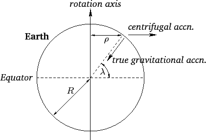It is convenient to define Cartesian axes in the rotating reference frame such that the $z'$-axis points vertically upward, and $x'$- and $y'$-axes are horizontal, with the $x'$-axis pointing directly northward, and the $y'$-axis pointing directly westward--see Figure 24. The Cartesian components of the Earth's angular velocity are thus

$$\mbox{\boldmath$\Omega$}= {\mit\Omega}\,(\cos\lambda,\,0,\,\sin\lambda),$$ (418)

whilst the vectors ${\bf R}$ and ${\bf g}$ are written

$${\bf R} = (0,\,0,\,R),$$ (419)

$${\bf g} = (0,\,0,\,-g),$$ (420)

respectively. It follows that the Cartesian coordinates of the apparent gravitational acceleration, (417), are

$${\bf g}' = \left(-{\mit\Omega}^2\,R\,\cos\lambda\,\sin\lambda,\,0,\, -g + {\mit\Omega}^2\,R\,\cos^2\lambda\right).$$ (421)

The magnitude of this acceleration is approximately

$$g' \simeq g - {\mit\Omega}^2\,R\,\cos^2\lambda \simeq 9.8 - 0.034\,\cos^2\lambda\,\,\, {\rm m/s^2}.$$ (422)

According to the above equation, the centrifugal acceleration causes the magnitude of the apparent gravitational acceleration on the Earth's surface to vary by about $0.3\%$, being largest at the poles, and smallest at the equator. This variation in apparent gravitational acceleration, due (ultimately) to the Earth's rotation, causes the Earth itself to bulge slightly at the equator (see Section 12.6), which has the effect of further intensifying the variation, since a point on the surface of the Earth at the equator is slightly further away from the Earth's center than a similar point at one of the poles (and, hence, the true gravitational acceleration is slightly weaker in the former case).

Another consequence of centrifugal acceleration is that the apparent gravitational acceleration on the Earth's surface has a horizontal component aligned in the north/south direction. This horizontal component ensures that the apparent gravitational acceleration does not point directly toward the center of the Earth. In other words, a plumb-line on the surface of the Earth does not point vertically downward, but is deflected slightly away from a true vertical in the north/south direction. The angular deviation from true vertical can easily be calculated from Equation (421):

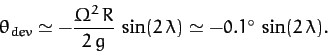$$\theta_{dev} \simeq - \frac{{\mit\Omega}^2\,R}{2\,g}\,\sin(2\,\lambda)\simeq -0.1^\circ\,\sin(2\,\lambda).$$ (423)

Here, a positive angle denotes a northward deflection, and vice versa. Thus, the deflection is southward in the northern hemisphere (i.e., $\lambda>0$) and northward in the southern hemisphere (i.e., $\lambda < 0$). The deflection is zero at the poles and at the equator, and reaches its maximum magnitude (which is very small) at middle latitudes.