An ellipse, centered on the origin, of major radius ![]() and minor radius
and minor radius ![]() , which are aligned
along the
, which are aligned
along the ![]() - and
- and ![]() -axes, respectively (see Figure 14), satisfies the following
well-known equation:
-axes, respectively (see Figure 14), satisfies the following
well-known equation:
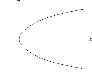
Likewise, a parabola which is aligned along the ![]() -axis, and passes through
the origin (see Figure 15), satisfies:
-axis, and passes through
the origin (see Figure 15), satisfies:
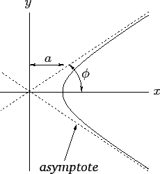
Finally, a hyperbola which is aligned along the ![]() -axis, and whose
asymptotes intersect at the origin (see Figure 16), satisfies:
-axis, and whose
asymptotes intersect at the origin (see Figure 16), satisfies:
It is not clear, at this stage, what the ellipse, the parabola, and the hyperbola
have in common (other than being conic sections). Well, it turns out that what these three curves
have in common is that they can all be represented as the locus of a movable point whose distance from
a fixed point is in a constant ratio to its perpendicular distance to some
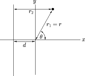
fixed straight-line. Let the fixed point (which is termed the focus
of the ellipse/parabola/hyperbola) lie at the origin, and let
the fixed line correspond to ![]() (with
(with ![]() ). Thus, the distance of a general point (
). Thus, the distance of a general point (![]() ,
, ![]() ) (which lies to the right of the line
) (which lies to the right of the line ![]() ) from the origin is
) from the origin is
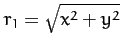 , whereas the perpendicular distance of the point from
the line
, whereas the perpendicular distance of the point from
the line ![]() is
is ![]() --see Figure 17.
In polar coordinates,
--see Figure 17.
In polar coordinates, ![]() and
and
![]() .
Hence, the locus of a point for which
.
Hence, the locus of a point for which
![]() and
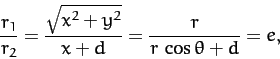
and ![]() are in a fixed ratio satisfies the following equation:
are in a fixed ratio satisfies the following equation:
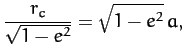
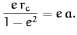
When written in terms of Cartesian coordinates, (233)
can be rearranged to give
When again written in terms of Cartesian coordinates, Equation (233)
can be rearranged to give
| (239) |
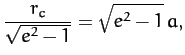
Finally, when written in terms of Cartesian coordinates, Equation (233)
can be rearranged to give
 |
(241) | ||
 |
(242) | ||
 |
(243) |
 |
(244) |
In conclusion, Equation (234) is the polar equation of a general conic
section which is confocal with the origin. For ![]() , the conic section
is an ellipse. For
, the conic section
is an ellipse. For ![]() , the conic section is a parabola. Finally, for
, the conic section is a parabola. Finally, for
![]() , the conic section is a hyperbola.
, the conic section is a hyperbola.