


Next: Polar Coordinates
Up: Planetary Motion
Previous: Newtonian Gravity
Now gravity is a conservative force. Hence, the gravitational force (210) can be written (see Section 2.5)
 |
(213) |
where the potential energy,  , of our planet in the Sun's gravitational field takes the form
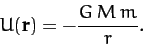 |
(214) |
It follows that the total energy of our planet is a conserved quantity--see Section 2.5. In other words,
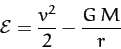 |
(215) |
is constant in time. Here,  is actually the planet's total energy per unit
mass, and
is actually the planet's total energy per unit
mass, and
 .
.
Gravity is also a central force. Hence, the angular momentum
of our planet is a conserved quantity--see Section 2.6. In other
words,
 |
(216) |
which is actually the planet's angular momentum per unit mass, is constant
in time. Taking the scalar product of the above equation with  , we
obtain
, we
obtain
 |
(217) |
This is the equation of a plane which passes through the origin, and
whose normal is parallel to  . Since is a constant vector,
it always points in the same direction. We, therefore, conclude that
the motion of our planet is two-dimensional in nature: i.e., it is confined to some fixed plane which passes through the origin. Without loss of generality, we can let this plane coincide with the
. Since is a constant vector,
it always points in the same direction. We, therefore, conclude that
the motion of our planet is two-dimensional in nature: i.e., it is confined to some fixed plane which passes through the origin. Without loss of generality, we can let this plane coincide with the  -
- plane.
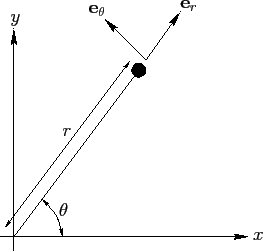
Figure 13:
Polar coordinates.
 |
Next: Polar Coordinates
Up: Planetary Motion
Previous: Newtonian Gravity
Richard Fitzpatrick
2011-03-31