


Next: Conservation Laws
Up: Planetary Motion
Previous: Kepler's Laws
Newtonian Gravity
The force which maintains the Planets in orbit around the Sun is
called gravity, and was first correctly described by Isaac
Newton (in 1687). According to Newton, any two point mass objects (or spherically
symmetric objects of finite extent)
exert a force of attraction on one another. This force points along the
line of centers joining the objects, is directly proportional to the product
of the objects' masses, and inversely proportional to the square of the distance between them. Suppose that the first object is the Sun, which is of mass  ,
and is located at the origin of our coordinate system. Let the
second object be some planet, of mass
,
and is located at the origin of our coordinate system. Let the
second object be some planet, of mass  , which is located
at position vector
, which is located
at position vector  . The gravitational force exerted on the
planet by the Sun is thus written
. The gravitational force exerted on the
planet by the Sun is thus written
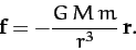 |
(210) |
The constant of proportionality,  , is called the gravitational constant,
and takes the value
, is called the gravitational constant,
and takes the value
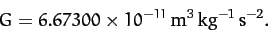 |
(211) |
An equal and opposite force to (210) acts on the Sun. However, we shall assume that
the Sun is so much more massive than the planet in question that this force does not
cause the Sun's position to shift appreciably. Hence, the Sun will always remain
at the origin of our coordinate system. Likewise, we shall neglect the
gravitational forces exerted on our planet by the other planets in the Solar System, compared to the much larger gravitational
force exerted by the Sun.
Incidentally, there is something rather curious about Equation (210). According to
this law, the gravitational force acting on an object is directly proportional
to its inertial mass. But why should inertia be related to the force of
gravity? After all, inertia measures the reluctance of a given body to
deviate from its preferred state of uniform motion in a straight-line,
in response to some external force. What has this got to do with gravitational
attraction?
This question perplexed physicists for many years, and was only
answered when Albert Einstein published his general theory of relativity
in 1916. According to Einstein, inertial mass acts as a sort
of gravitational charge since it impossible to distinguish
an acceleration produced by a gravitational field from an apparent acceleration
generated by observing in a non-inertial reference frame. The assumption that these
two types of acceleration are indistinguishable leads directly to all
of the strange predictions of general relativity: e.g.,
clocks in different gravitational potentials run at different rates,
mass bends space, etc.
According to Equation (210), and Newton's second law, the equation
of motion of our planet takes the form
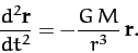 |
(212) |
Note that the planetary mass, , has canceled out on both sides of
the above equation.
Next: Conservation Laws
Up: Planetary Motion
Previous: Kepler's Laws
Richard Fitzpatrick
2011-03-31