The directions of the three mutually orthogonal unit vectors
![]() define the three so-called principal axes
of rotation of the rigid body under investigation. These axes are special because when the body rotates about
one of them (i.e., when
define the three so-called principal axes
of rotation of the rigid body under investigation. These axes are special because when the body rotates about
one of them (i.e., when ![]() is parallel to one of them) the angular momentum vector
is parallel to one of them) the angular momentum vector ![]() becomes parallel to the angular velocity vector
becomes parallel to the angular velocity vector ![]() .
This can be seen from a comparison of Equation (466) and Equation (487).
.
This can be seen from a comparison of Equation (466) and Equation (487).
Suppose that we reorient our Cartesian coordinate
axes so the they coincide with the mutually orthogonal principal axes of rotation. In this new reference frame, the eigenvectors of ![]() are the unit vectors,
are the unit vectors,
![]() ,
, ![]() , and
, and ![]() , and the eigenvalues
are the moments of inertia about these axes,
, and the eigenvalues
are the moments of inertia about these axes, ![]() ,
, ![]() , and
, and ![]() , respectively. These latter quantities are referred to as the
principal moments of inertia.
Note that the products of inertia are all zero in the new
reference frame. Hence, in this frame, the moment
of inertia tensor takes the form of a diagonal matrix: i.e.,
, respectively. These latter quantities are referred to as the
principal moments of inertia.
Note that the products of inertia are all zero in the new
reference frame. Hence, in this frame, the moment
of inertia tensor takes the form of a diagonal matrix: i.e.,
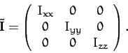 |
(488) |
When expressed in our new coordinate system, Equation (466)
yields
| (489) |
| (490) |
In conclusion, there are many great simplifications to be had by choosing a coordinate system whose axes coincide with the principal axes of rotation of the rigid body under investigation. But how do we determine the directions of the principal axes in practice?
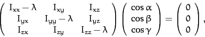
Well, in general, we have to solve the eigenvalue equation
| (491) |
Fortunately, however, in many instances the rigid body under investigation possesses some kind of symmetry, so that at least one principal axis can be found by inspection. In this case, the other two principal axes can be determined as follows.
Suppose that the ![]() -axis is known to be a principal axes (at the origin)
in some coordinate system. It follows that the two products of inertia
-axis is known to be a principal axes (at the origin)
in some coordinate system. It follows that the two products of inertia ![]() and
and ![]() are zero [otherwise,
are zero [otherwise, ![]() would not be an eigenvector in Equation (492)]. The other two principal axes must lie in the
would not be an eigenvector in Equation (492)]. The other two principal axes must lie in the
![]() -
-![]() plane: i.e.,
plane: i.e., ![]() . It then follows that
. It then follows that
![]() , since
, since
![]() .
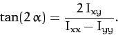
The first two rows in the matrix equation (492) thus
reduce to
.
The first two rows in the matrix equation (492) thus
reduce to
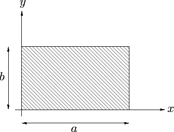
As an example, consider a uniform rectangular lamina of mass ![]() and sides
and sides ![]() and
and ![]() which lies
in the
which lies
in the ![]() -
-![]() plane, as shown in Figure 29. Suppose that the axis of
rotation passes through the origin (i.e., through a corner of the lamina).
Since
plane, as shown in Figure 29. Suppose that the axis of
rotation passes through the origin (i.e., through a corner of the lamina).
Since ![]() throughout the lamina, it follows from Equations (464) and
(465) that
throughout the lamina, it follows from Equations (464) and
(465) that
![]() . Hence, the
. Hence, the ![]() -axis
is a principal axis. After some straightforward integration, Equations (460)-(463) yield
-axis
is a principal axis. After some straightforward integration, Equations (460)-(463) yield
 |
(497) | ||
 |
(498) | ||
 |
(499) |
 |
(500) |