


Next: McCullough's Formula
Up: Gravitational Potential Theory
Previous: Potential Outside a Uniform
Rotational Flattening
Let us consider the equilibrium configuration of a self-gravitating spheroid,
composed of uniform density incompressible fluid, which is rotating
steadily
about some fixed axis. Let  be the total mass,
  the mean radius,
 the ellipticity, and
  the angular velocity of rotation. Furthermore, let the axis of rotation coincide with the axis of symmetry, which is assumed to run along the
  -axis.
Let us transform to a non-inertial frame of reference which co-rotates with the spheroid about the -axis, and in which the spheroid consequently appears to be stationary. From Chapter 7,
the problem is now analogous to that of a non-rotating spheroid, except that
the surface acceleration is written
 ,
where
,
where
 is the gravitational acceleration, and
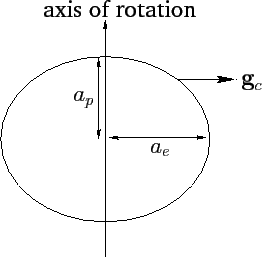
 the centrifugal acceleration. The latter acceleration
is of magnitude
the centrifugal acceleration. The latter acceleration
is of magnitude
 , and is everywhere directed
away from the axis of rotation (see Figure 40 and Chapter 7).
The acceleration thus has components
, and is everywhere directed
away from the axis of rotation (see Figure 40 and Chapter 7).
The acceleration thus has components
 |
|
|
(912) |
in spherical polar coordinates. It follows that
 ,
where
,
where
![\begin{displaymath}
\chi(r,\theta) = - \frac{\Omega^2\,r^2}{2}\,\sin^2\theta= -\frac{\Omega^2\,r^2}{3}\,\left[1-P_2(\cos\theta)\right]
\end{displaymath}](img2170.png) |
(913) |
can be thought of as a sort of centrifugal potential. Hence, the
total surface acceleration is
 |
(914) |
As before, the criterion for an equilibrium state is that the surface lie at
a constant total potential, so as to eliminate tangential surface forces which
cannot be balanced by internal pressure. Hence, assuming that the
surface satisfies Equation (901), the equilibrium configuration is specified by
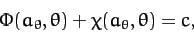 |
(915) |
where  is a constant. It follows from Equations (911) and (913) that, to first-order in and
 ,
,
![\begin{displaymath}
- \frac{G\,M}{a} \left[1+ \frac{4}{15}\,\epsilon\,P_2(\cos\t...
...c{\mit\Omega^2\,a^2}{3}\left[1-P_2(\cos\theta)\right]\simeq c,
\end{displaymath}](img2173.png) |
(916) |
which yields
 |
(917) |
We conclude, from the above expression, that the equilibrium configuration
of a (relatively slowly) rotating self-gravitating mass distribution is an oblate spheroid: i.e., a sphere
which is slightly flattened along its axis of rotation. The degree of flattening is proportional
to the square of the rotation rate. Now, from (901), the mean radius
of the spheroid is
, the radius at the poles (i.e., along the axis of rotation) is
 , and the radius at the
equator (i.e., perpendicular to the axis of rotation) is
, and the radius at the
equator (i.e., perpendicular to the axis of rotation) is
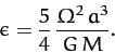
 --see Figure 40. Hence, the degree of rotational flattening
can be written
--see Figure 40. Hence, the degree of rotational flattening
can be written
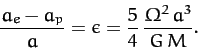 |
(918) |
Figure 40:
Rotational flattening.
 |
Now, for the Earth,
 ,
,
 , and
, and
 .
Thus, we predict that
.
Thus, we predict that
 |
(919) |
corresponding to a difference between equatorial and polar radii
of
 |
(920) |
In fact, the observed degree of flattening of the Earth is
 ,
corresponding to a difference between equatorial and polar radii
of
,
corresponding to a difference between equatorial and polar radii
of
 . The main reason that our analysis has overestimated the
degree of rotational flattening of the Earth is that it models the terrestrial interior as a uniform density incompressible fluid. In reality,
the Earth's core is much denser than its crust (see Exercise 12.1).
. The main reason that our analysis has overestimated the
degree of rotational flattening of the Earth is that it models the terrestrial interior as a uniform density incompressible fluid. In reality,
the Earth's core is much denser than its crust (see Exercise 12.1).
For Jupiter,
 ,
,
 , and
, and
 . Hence,
we predict that
. Hence,
we predict that
 |
(921) |
Note that this degree of flattening is much larger than that of the Earth, due to
Jupiter's relatively large radius (about 10 times that of Earth), combined with its relatively
short rotation period (about 0.4 days). In fact, the polar flattening of
Jupiter is clearly apparent from images of this planet. The observed degree of
polar flattening of Jupiter is actually
 . Our estimate of is probably
slightly too large because Jupiter, which is mostly gaseous, has a mass distribution which is strongly concentrated
at its core (see Exercise 12.1).
. Our estimate of is probably
slightly too large because Jupiter, which is mostly gaseous, has a mass distribution which is strongly concentrated
at its core (see Exercise 12.1).
Next: McCullough's Formula
Up: Gravitational Potential Theory
Previous: Potential Outside a Uniform
Richard Fitzpatrick
2011-03-31