


Next: Axisymmetric Incompressible Inviscid Flow
Up: Two-Dimensional Potential Flow
Previous: Blasius Theorem
- Demonstrate that a line source of strength
 (running along the
  -axis) situated in a uniform flow of (unperturbed) velocity
  (lying in the
  -
- plane) and density
  experiences a force per unit length
- Demonstrate that a vortex filament of intensity
 (running along the
-axis) situated in a uniform flow of (unperturbed) velocity
(lying in the
-
plane) and density
experiences a force per unit length
(running along the
-axis) situated in a uniform flow of (unperturbed) velocity
(lying in the
-
plane) and density
experiences a force per unit length
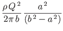
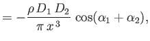
- Show that two parallel line sources of strengths
and
 , located a perpendicular distance
  apart, exert a radial
force per unit length
apart, exert a radial
force per unit length
 on one another, the force being attractive if
  , and
repulsive if
, and
repulsive if  .
.
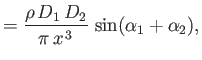
- Show that two parallel vortex filaments of intensities
and
 , located a perpendicular distance
apart, exert a radial
force per unit length
, located a perpendicular distance
apart, exert a radial
force per unit length
 on one another, the force being repulsive if
 , and
attractive if
, and
attractive if
 .
.
- A vortex filament of intensity
runs parallel to, and lies a perpendicular distance
 from, a rigid planar boundary. Demonstrate that
the boundary experiences a net force per unit length
from, a rigid planar boundary. Demonstrate that
the boundary experiences a net force per unit length
 directed toward the
filament.
directed toward the
filament.
- Two rigid planar boundaries meet at right-angles. A line source of strength
runs parallel to the line of intersection of the planes, and is situated a
perpendicular distance
from each. Demonstrate that the source is subject to a force per unit length
directed towards the line of intersection of the planes.
- A line source of strength
is located a distance
 from an impenetrable circular cylinder of radius
  (the axis
of the cylinder being parallel to the source). Demonstrate that the cylinder experiences a net force per unit length
(the axis
of the cylinder being parallel to the source). Demonstrate that the cylinder experiences a net force per unit length
directed toward the source.
- A dipole line source consists of a line source of strength
, running parallel to the
-axis, and intersecting the
-
plane at
 ,
,
 , and
a parallel source of strength
, and
a parallel source of strength  that intersects the
-
plane at
that intersects the
-
plane at
 ,
,
 . Show
that, in the limit
. Show
that, in the limit
 , and
, and
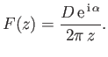
 , the complex velocity potential of the source is
Here,
 is termed the complex dipole strength.
- A dipole line source of complex strength
is placed in a uniformly flowing fluid
of speed
 whose direction of motion subtends a (counter-clockwise) angle
  with the
-axis.
Show that, while no net force acts on the source, it is subject to a moment (per unit length)
with the
-axis.
Show that, while no net force acts on the source, it is subject to a moment (per unit length)
 about the
-axis.
about the
-axis.
- Consider a dipole line source of complex strength
 running along the
-axis,
and a second parallel source of complex strength
running along the
-axis,
and a second parallel source of complex strength
 that intersects the
-
plane
at
that intersects the
-
plane
at  ,
,  .
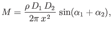
Demonstrate that the first source is subject to a moment (per unit length) about the
-axis of
.
Demonstrate that the first source is subject to a moment (per unit length) about the
-axis of
as well as a force (per unit length) whose
- and
-components are
respectively. Show that the second source is subject to the same moment, but an equal and opposite force.
- A dipole line source of complex strength
runs parallel to, and is located a
perpendicular distance
from, a rigid planar boundary. Show that the
boundary experiences a force per unit length
acting toward the source.
- Demonstrate that a conformal map converts a line source into a line source of the same strength, and
a vortex filament into a vortex filament of the same intensity.
- Consider the conformal map
where
 ,
,
 , and
, and  is real and positive. Show that
Demonstrate that  , where
 , maps to a circular arc of center
  ,
,
 , and
radius
, and
radius
 , that connects the points
  ,
, and lies in the region
,
, and lies in the region  . Demonstrate that
 maps to the continuation of this arc in the region
  . In particular, show that
  maps to the region
  on the
-axis, whereas
on the
-axis, whereas  maps to the region
  . Finally, show that
 maps to a circle of center
 ,
, and radius
,
, and radius
 .
.
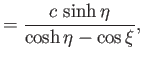
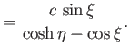
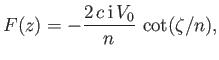
- Consider the complex velocity potential
where
Here,
,  , and
are real and positive. Show that
, and
are real and positive. Show that
Hence, deduce that the flow at
 is uniform,
parallel to the
-axis, and of speed
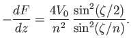
. Demonstrate that
is uniform,
parallel to the
-axis, and of speed
. Demonstrate that
Hence, deduce that the streamline  runs along the
-axis for
, but along a
circular arc connecting the points
,
for
. Furthermore, show that if
runs along the
-axis for
, but along a
circular arc connecting the points
,
for
. Furthermore, show that if  then this arc lies above the
-axis, and is of maximum height
then this arc lies above the
-axis, and is of maximum height
but if  then the arc lies below the
-axis, and is of maximum depth
then the arc lies below the
-axis, and is of maximum depth
Hence, deduce that if
then the complex velocity potential under investigation corresponds to uniform flow of speed
,
parallel to a planar boundary that possesses
a cylindrical bump (whose axis is normal to the flow) of height  and width
  , but if
then the potential corresponds to flow parallel to a planar
boundary that possesses a cylindrical depression of depth
, but if
then the potential corresponds to flow parallel to a planar
boundary that possesses a cylindrical depression of depth  and width
. Show, in particular, that if
and width
. Show, in particular, that if  then
the bump is a half-cylinder, and if
then
the bump is a half-cylinder, and if  then the depression is a half-cylinder. Finally, demonstrate that the
flow speed at the top of the bump (in the case
), or the bottom of the depression (in the case
) is
then the depression is a half-cylinder. Finally, demonstrate that the
flow speed at the top of the bump (in the case
), or the bottom of the depression (in the case
) is
- Show that
 maps the semi-infinite strip
 ,
,  in the
  -plane
onto the upper half (
-plane
onto the upper half ( ) of the
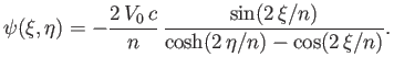
-plane. Hence, show that the stream function due to a line source of strength
placed at
) of the
-plane. Hence, show that the stream function due to a line source of strength
placed at
 ,
,  , in the rectangular region
,
bounded by the rigid planes
, in the rectangular region
,
bounded by the rigid planes
 ,
, and
,
, and  , is
, is
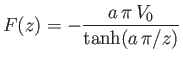
- Show that the complex velocity potential
can be interpreted as that due to uniform flow of speed
over a cylindrical log of radius
lying on the flat bed of a deep
stream (the axis of the log being normal to the flow).
Demonstrate that the flow speed at the top of the log is
 . Finally, show that the pressure
difference between the top and bottom of the log is
. Finally, show that the pressure
difference between the top and bottom of the log is
 .
.
- Show that the complex potential
where
( ) represents uniform flow of unperturbed speed
  , whose direction subtends a (counter-clockwise) angle
  with
the
-axis, around an impenetrable elliptic cylinder of major radius
with
the
-axis, around an impenetrable elliptic cylinder of major radius
 , aligned along the
-axis, and
minor radius
, aligned along the
-axis, and
minor radius
 , aligned along the
-axis. Demonstrate that the moment per unit length (about the
-axis)
exerted on the cylinder by the flow is
, aligned along the
-axis. Demonstrate that the moment per unit length (about the
-axis)
exerted on the cylinder by the flow is
Hence, deduce that the moment acts to turn the cylinder broadside-on to the flow (i.e.,
 is a dynamically stable
equilibrium state), and that the equilibrium state in which the cylinder is aligned with the flow (i.e.,
is a dynamically stable
equilibrium state), and that the equilibrium state in which the cylinder is aligned with the flow (i.e.,  ) is
dynamically unstable.
) is
dynamically unstable.
- Consider a simply-connected region of a two-dimensional flow pattern bounded on the inside by the closed curve
 (lying in the
-
plane), and on the
outside by the closed curve
(lying in the
-
plane), and on the
outside by the closed curve  . Here,
and
do not necessarily correspond to streamlines of the flow. Demonstrate that the kinetic energy per unit
length (in the
-direction) of the fluid lying between the two curves is
. Here,
and
do not necessarily correspond to streamlines of the flow. Demonstrate that the kinetic energy per unit
length (in the
-direction) of the fluid lying between the two curves is
where
is the fluid mass density,  the velocity potential, and
  the stream function. Here,
  is a curve that runs from
to
, and
is a curve that runs from
to
, and ![$ [\phi]$](img2510.png) denotes the amount by which the velocity potential increases as the
argument of
denotes the amount by which the velocity potential increases as the
argument of
 increases by
  .
.
- Show that the complex potential
where
(
) represents the flow pattern around an impenetrable elliptic cylinder of major radius
, aligned along the
-axis, and
minor radius
, aligned along the
-axis, moving with speed
, in a direction that makes a counter-clockwise angle
with the
-axis, through a fluid that is at rest far from the cylinder. Demonstrate that the kinetic energy per unit length of the
flow pattern is
where
is the fluid mass density.
Hence, show that the cylinder's added mass per unit length is
- Demonstrate from Equation (6.110) that the equation of the free streamline
 , in the case of a liquid jet emerging from
a two-dimensional orifice of semi-width
formed by a gap between two semi-infinite plane walls that subtend an angle
, in the case of a liquid jet emerging from
a two-dimensional orifice of semi-width
formed by a gap between two semi-infinite plane walls that subtend an angle  , can be written parametrically
as:
, can be written parametrically
as:
where
 . Here, the orifice corresponds to the plane
  , and the flow a long way from the orifice is in the
  -direction.
Show that for the case of a two-dimensional Borda mouthpiece,
-direction.
Show that for the case of a two-dimensional Borda mouthpiece,
 , the previous equations reduce to
Finally, show that the previous equations predict that the free streamline is re-entrant, with  attaining its minimum value
 when
when
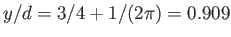 .
.
Next: Axisymmetric Incompressible Inviscid Flow
Up: Two-Dimensional Potential Flow
Previous: Blasius Theorem
Richard Fitzpatrick
2016-03-31


![$\displaystyle h = c\left[\frac{\cos(\pi\,n/2)+1}{\sin(\pi\,n/2)}\right],
$](img2484.png)
![$\displaystyle d = c\left[\frac{\cos(\pi\,n/2)+1}{\vert\sin(\pi\,n/2)\vert}\right].
$](img2486.png)
![$\displaystyle v = \frac{2\,V_0}{n^{\,2}}\left[1-\cos(\pi\,n/2)\right].
$](img2490.png)
![$\displaystyle \psi(\xi,\eta) = \frac{Q\,\sinh(\pi\,\xi/a)\,\sin(\pi\,\eta/a)}{2\pi\,[\sinh^2(\pi\,\xi/a)+\cos^2(\pi\,\eta/a)]}.
$](img2497.png)

![$\displaystyle K= \frac{1}{2}\,\rho\left[\int_{C_2}\phi\,d\psi-\int_{C_1}\phi\,d\psi-\int_{C_3}[\phi]\,d\psi\right],
$](img2508.png)
![$\displaystyle =\frac{2}{\pi}\int_{\sin^{-1}(\lambda)}^{\pi/2}\cos\left(\frac{2\...
...left(\frac{2\,\alpha}{\pi}\,\beta\right)\frac{d\beta}{\tan\beta}\right]^{\,-1},$](img2516.png)
![$\displaystyle =1-\frac{2}{\pi}\int_{\sin^{-1}(\lambda)}^{\pi/2}\sin\left(\frac{...
...left(\frac{2\,\alpha}{\pi}\,\beta\right)\frac{d\beta}{\tan\beta}\right]^{\,-1},$](img2517.png)
![$\displaystyle = \frac{1}{\pi}\left[-\ln(\lambda)-1+\lambda^{\,2}\right],$](img2519.png)
![$\displaystyle = \frac{1}{2}+\frac{1}{\pi}\left[\sin^{-1}(\lambda)+\lambda\,(1-\lambda^{\,2})^{1/2}\right].$](img2520.png)