


Next: Capillary Curves
Up: Surface Tension
Previous: Angle of Contact
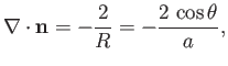
Consider a situation in which a narrow, cylindrical, glass tube of radius  is
dipped vertically into a liquid of density
is
dipped vertically into a liquid of density  , and the liquid level within the tube rises a height
  above the free surface
as a consequence of surface tension. (See Figure 3.3.) Suppose that the radius of the
tube is much less than the capillary length. A tube for which this is the case is generally
known as a capillary tube.
According to the discussion in Section 3.4, the shape of the internal liquid/air interface within a capillary tube
is not significantly affected by gravity. Thus, from Section 3.3, the interface is
a segment of a sphere of radius
above the free surface
as a consequence of surface tension. (See Figure 3.3.) Suppose that the radius of the
tube is much less than the capillary length. A tube for which this is the case is generally
known as a capillary tube.
According to the discussion in Section 3.4, the shape of the internal liquid/air interface within a capillary tube
is not significantly affected by gravity. Thus, from Section 3.3, the interface is
a segment of a sphere of radius  (say). If
  is the angle of contact of interface with the glass then simple geometry (see Figure 3.3) reveals that
 |
(3.20) |
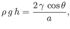
Hence, from Equation (3.13), the mean curvature of the interface is given by
 |
(3.21) |
where  is the associated surface tension. [The minus sign in the previous expression arises from the
fact that
is the associated surface tension. [The minus sign in the previous expression arises from the
fact that  points towards the center of curvature of the interface, whereas the opposite is true for Equation (3.13).] Finally, from
Equation (3.15), application of the Young-Laplace equation to the interface yields
points towards the center of curvature of the interface, whereas the opposite is true for Equation (3.13).] Finally, from
Equation (3.15), application of the Young-Laplace equation to the interface yields
 |
(3.22) |
which can be rearranged to give
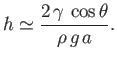 |
(3.23) |
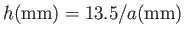
This result, which relates the height,
, to which a liquid rises in a capillary tube of radius
to the
liquid's surface tension,
, is known as Jurin's law, and is named after its discoverer, James Jurin (1684-1750).
The assumption that the radius of the tube is much less than the capillary length
is equivalent to the assumption that the height of the interface above the free surface of the
liquid is much greater than the radius of the tube.
This follows, from Equations (3.16) and (3.23), because
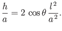 |
(3.24) |
Thus, the ordering  implies that
  .
.
For the case of water at  , assuming a contact angle of
  , Jurin's law yields
 (Batchelor 2000). Thus, water rises a height
 in a capillary tube of
radius
in a capillary tube of
radius
 , but rises
 in a capillary tube of radius
 .
In the case of a liquid, such a mercury, that has an oblique
angle of contact with glass, so that
.
In the case of a liquid, such a mercury, that has an oblique
angle of contact with glass, so that
 , the liquid level in a capillary tube is depressed
below that of the free surface (i.e.,
, the liquid level in a capillary tube is depressed
below that of the free surface (i.e.,  ).
).
Next: Capillary Curves
Up: Surface Tension
Previous: Angle of Contact
Richard Fitzpatrick
2016-03-31