Momentum Conservation

Consider a fixed volume $V$ surrounded by a surface $S$ . The $i$ -component of the total linear momentum contained within $V$ is

$$P_i = \int_V \rho\,v_i\,dV.$$ (1.43)

Moreover, the flux of $i$ -momentum across $S$ , and out of $V$ , is [see Equation (1.29)]

$${\mit\Phi}_i = \oint_S \rho\,v_i\,v_j\,dS_j.$$ (1.44)

Finally, the $i$ -component of the net force acting on the fluid within $V$ is

$$f_i = \int_V F_i\,dV + \oint_S \sigma_{ij}\,dS_j,$$ (1.45)

where the first and second terms on the right-hand side are the contributions from volume and surface forces, respectively.

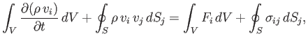
Momentum conservation requires that the rate of increase of the net $i$ -momentum of the fluid contained within $V$ , plus the flux of $i$ -momentum out of $V$ , is equal to the rate of $i$ -momentum generation within $V$ . Of course, from Newton's second law of motion, the latter quantity is equal to the $i$ -component of the net force acting on the fluid contained within $V$ . Thus, we obtain [cf., Equation (1.31)]

$$\frac{dP_i}{dt} + {\mit\Phi}_i = f_i,$$ (1.46)

which can be written

$$\int_V \frac{\partial(\rho\,v_i)}{\partial t}\,dV +\oint_S\rho\,v_i\,v_j\,dS_j = \int_V F_i\,dV + \oint_S \sigma_{ij}\,dS_j,$$ (1.47)

because the volume $V$ is non-time-varying. Making use of the tensor divergence theorem, this becomes

$$\int_V\left[\frac{\partial (\rho\,v_i)}{\partial t} + \frac{\part... ...right]dV = \int_V\left(F_i + \frac{\partial\sigma_{ij}}{\partial x_j}\right)dV.$$ (1.48)

However, the previous result is valid irrespective of the size, shape, or location of volume $V$ , which is only possible if

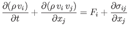$$\frac{\partial (\rho\,v_i)}{\partial t} + \frac{\partial(\rho\,v_i\,v_j)}{\partial x_j} = F_i + \frac{\partial\sigma_{ij}}{\partial x_j}$$ (1.49)

everywhere inside the fluid. Expanding the derivatives, and rearranging, we obtain

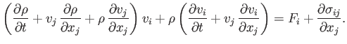$$\left(\frac{\partial\rho}{\partial t} + v_j\,\frac{\partial\rho}{... ...tial v_i}{\partial x_j}\right)= F_i + \frac{\partial\sigma_{ij}}{\partial x_j}.$$ (1.50)

In tensor notation, the continuity equation (1.37) is written

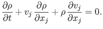$$\frac{\partial\rho}{\partial t} + v_j\,\frac{\partial\rho}{\partial x_j} + \rho\,\frac{\partial v_j}{\partial x_j}=0.$$ (1.51)

So, combining Equations (1.50) and (1.51), we obtain the following fluid equation of motion,

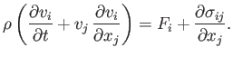$$\rho\left(\frac{\partial v_i}{\partial t} + v_j\,\frac{\partial v_i}{\partial x_j}\right)= F_i + \frac{\partial\sigma_{ij}}{\partial x_j}.$$ (1.52)

An alternative form of this equation is

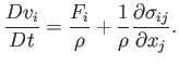$$\frac{D v_i}{Dt} = \frac{F_i}{\rho} + \frac{1}{\rho}\frac{\partial\sigma_{ij}}{\partial x_j}.$$ (1.53)

The previous equation describes how the net volume and surface forces per unit mass acting on a co-moving fluid element determine its acceleration.