


Next: Equations of Incompressible Fluid
Up: Mathematical Models of Fluid
Previous: Navier-Stokes Equation
Consider a fixed volume  surrounded by a surface
  . The total energy content of the fluid contained within
is
. The total energy content of the fluid contained within
is
 |
(1.59) |
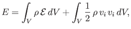
where the first and second terms on the right-hand side are the net internal and kinetic energies, respectively. Here,
 is the internal (i.e., thermal) energy per unit mass of the fluid. The energy flux
across
, and out of
, is [cf., Equation (1.29)]
is the internal (i.e., thermal) energy per unit mass of the fluid. The energy flux
across
, and out of
, is [cf., Equation (1.29)]
![$\displaystyle {\mit\Phi}_E = \oint_S \rho\left({\cal E} + \frac{1}{2}\,v_i\,v_i...
...ial x_j}\! \left[\rho\left({\cal E} + \frac{1}{2}\,v_i\,v_i\right)v_j\right]dV,$](img288.png) |
(1.60) |
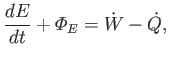
where use has been made of the tensor divergence theorem. According to the first law of thermodynamics, the rate of increase of
the energy contained within
, plus the net energy flux out of
, is equal to the net rate of work done on the fluid
within
, minus the
net heat flux out of
: that is,
 |
(1.61) |
where  is the net rate of work, and
  the net heat flux. It can be seen that
 is the
effective energy generation rate within
[cf., Equation (1.31)].
is the
effective energy generation rate within
[cf., Equation (1.31)].
The net rate at which volume and surface forces do work on the fluid within
is
![$\displaystyle \dot{W} = \int_V v_i\,F_i\,dV + \oint_S v_i\,\sigma_{ij}\,dS_j = \int_V\left[v_i\,F_i+ \frac{\partial(v_i\,\sigma_{ij})}{\partial x_j}\right]dV,$](img293.png) |
(1.62) |
where use has been made of the tensor divergence theorem.
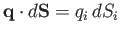
Generally speaking, heat flow in fluids is driven by temperature gradients. Let the
 be the
Cartesian components of the heat flux density at position
be the
Cartesian components of the heat flux density at position  and time
  . It follows that the heat flux
across a surface element
. It follows that the heat flux
across a surface element  , located at point
, is
, located at point
, is
 . Let
. Let
 be
the temperature of the fluid at position
and time
. Thus, a general temperature gradient takes the
form
be
the temperature of the fluid at position
and time
. Thus, a general temperature gradient takes the
form
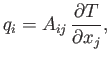
 . Let us assume that there is a linear relationship between the components of the local heat flux
density and the local temperature gradient: that is,
. Let us assume that there is a linear relationship between the components of the local heat flux
density and the local temperature gradient: that is,
 |
(1.63) |
where the  are the components of a second-rank tensor (which can be functions of position and time).
In an isotropic fluid we would expect
to be an isotropic tensor. (See Section B.5.)
However, the most general second-order isotropic tensor is simply a multiple of
are the components of a second-rank tensor (which can be functions of position and time).
In an isotropic fluid we would expect
to be an isotropic tensor. (See Section B.5.)
However, the most general second-order isotropic tensor is simply a multiple of
 . Hence, we can write
 |
(1.64) |
where
 is termed the thermal conductivity of the fluid. It follows that the most general
expression for the heat flux density in an isotropic fluid is
is termed the thermal conductivity of the fluid. It follows that the most general
expression for the heat flux density in an isotropic fluid is
 |
(1.65) |
or, equivalently,
 |
(1.66) |
Moreover, it is a matter of experience that heat flows down temperature gradients: that is,  .
We conclude that the net heat flux out of volume
is
.
We conclude that the net heat flux out of volume
is
 |
(1.67) |
where use has been made of the tensor divergence theorem.
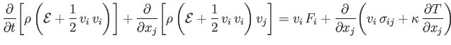
Equations (1.59)-(1.62) and (1.67) can be combined to give the following energy conservation equation:
![$\displaystyle \int_V\left\{\frac{\partial}{\partial t}\!\left[\rho\left({\cal E...
...x_j}\!\left[\rho\left({\cal E}+\frac{1}{2}\,v_i\,v_i\right)v_j\right]\right\}dV$](img306.png) |
|
![$\displaystyle = \int_V\left[v_i\,F_i + \frac{\partial}{\partial x_j}\!\left(v_i\,\sigma_{ij} + \kappa\,\frac{\partial T}{\partial x_j}\right)\right]dV.$](img307.png) |
|
(1.68) |
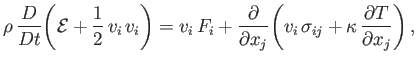
However, this result is valid irrespective of the size, shape, or location of volume
, which is only
possible if
 |
(1.69) |
everywhere inside the fluid. Expanding some of the derivatives, and rearranging, we obtain
 |
(1.70) |
where use has been made of the continuity equation, (1.40).
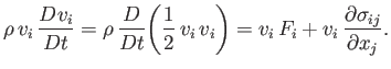
The scalar product of  with the fluid equation of motion, (1.53), yields
 |
(1.71) |
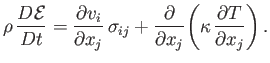
Combining the previous two equations, we get
 |
(1.72) |
Finally, making use of Equation (1.26), we deduce that the energy conservation equation for an isotropic Newtonian fluid
takes the general form
![$\displaystyle \frac{D{\cal E}}{Dt} = - \frac{p}{\rho}\,\frac{\partial v_i}{\par...
...l}{\partial x_j}\!\left( \kappa\,\frac{\partial T}{\partial x_j}\right)\right].$](img313.png) |
(1.73) |
Here,
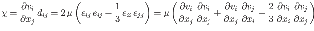 |
(1.74) |
is the rate of heat generation per unit volume due to viscosity.
When written in vector form, Equation (1.73) becomes
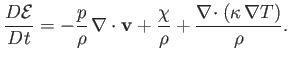 |
(1.75) |
According to the previous equation, the internal energy per unit mass of a co-moving fluid element
evolves in time as a consequence of work done on the element by pressure as
its volume changes, viscous heat generation due to flow shear, and heat conduction.
Next: Equations of Incompressible Fluid
Up: Mathematical Models of Fluid
Previous: Navier-Stokes Equation
Richard Fitzpatrick
2016-01-22