Example 2-d electrostatic calculation

Let us perform an example 2-d electrostatic calculation. Consider a charged wire running parallel to the axis of a uniform, hollow, rectangular, conducting channel. Suppose that the vertices of the channel lie at $(x,y) = (0,0)$, $(0,1)$, $(1,0)$, and $(1,1)$. Suppose, further, that the wire carries a uniform charge per unit length of magnitude unity. The electric potential $\phi(x,y)$ inside the channel satisfies [see Eq. (110)]

$$\frac{\partial^2 \phi(x,y)}{\partial x^2}+\frac{\partial^2 \... ...x,y)}{\partial y^2} = v(x,y) = -\delta(x-x_0)\, \delta(y-y_0),$$ (185)

where $(x_0, y_0)$ are the coordinates of the wire. Here, we have conveniently normalized our units such that the factor $\epsilon _0$ is absorbed into the normalization. Assuming that the box is grounded, the potential is subject to the Dirichlet boundary conditions $\phi =0$ at $x=0$, $x=1$, $y=0$, and $y=1$. We require the solution in the region $0\leq x\leq 1$ and $0\leq y \leq 1$.

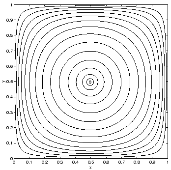
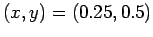
Figure 67: Contour plot of the electric potential generated by a charged wire placed at the center of a grounded rectangular channel. The wire is located at $(x,y)=(0.5,0.5)$, whereas the channel walls are at $x=0$, $x=1$, $y=0$, and $y=1$. Calculation performed with $N=J=128$.

Note that when discretizing Eq. (185) the right-hand side becomes

$$v(x_i, y_j) = -\frac{1}{\delta x\,\delta y}$$ (186)

on the grid-point closest to the wire, with $v(x_i, y_j) = 0$ on the remaining grid-points. Here, $\delta x$ and $\delta y$ are the grid spacings in the $x$- and $y$- directions, respectively.

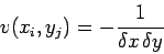
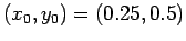
Figure 68: Vector plot showing the direction of the electric field generated by a charged wire placed at the center of a grounded rectangular channel. The wire is located at $(x,y)=(0.5,0.5)$, whereas the channel walls are at $x=0$, $x=1$, $y=0$, and $y=1$. Calculation performed with $N=J=128$.

Figures 67 and 68 show the electric potential $\phi(x,y)$ and electric field ${\bf E} = -\nabla \phi$ generated by a wire placed at the center of the channel: i.e., $(x_0,y_0) = (0.5,0.5)$. The calculation was performed with the previously listed 2-d Poisson solver using $N=J=128$.

Figure 69: Contour plot of the electric potential generated by a charged wire offset from the center of a grounded rectangular channel. The wire is located at $(x,y)=(0.25,0.5)$, whereas the channel walls are at $x=0$, $x=1$, $y=0$, and $y=1$. Calculation performed with $N=J=128$.

Figures 69 and 70 show the electric potential $\phi(x,y)$ and electric field ${\bf E} = -\nabla \phi$ generated by a wire offset from the center of the channel: i.e., $(x_0,y_0) = (0.25,0.5)$. The calculation was performed with the previously listed 2-d Poisson solver using $N=J=128$.

Figure 70: Vector plot showing the direction of the electric field generated by a charged wire offset from the center of a grounded rectangular channel. The wire is located at $(x,y)=(0.25,0.5)$, whereas the channel walls are at $x=0$, $x=1$, $y=0$, and $y=1$. Calculation performed with $N=J=128$.