| (102) | |||
| (103) |
According to the linear analysis of Sect. 4.2,
 |
(104) | ||
 |
(105) |
 |
 |
 |
 |
Figures 49-52 show the results of the experiment described above,
in which the pendulum's phase-space trajectory is moved slightly off an attractor
and the phase-space separation between the perturbed and unperturbed trajectories
is then monitored as a function of time,
at various stages on the period-doubling cascade discussed in the previous section.
To be more exact, the figures show the logarithm of the absolute magnitude of the
![]() -component of the phase-space separation between the perturbed and unperturbed
trajectories as a function of normalized time.
-component of the phase-space separation between the perturbed and unperturbed
trajectories as a function of normalized time.
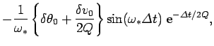
Figure 49 shows the time evolution of the ![]() -component of the phase-space
separation,
-component of the phase-space
separation, ![]() , between two neighbouring trajectories, one of which is the period-4
attractor illustrated in Fig. 45. It can be seen that
, between two neighbouring trajectories, one of which is the period-4
attractor illustrated in Fig. 45. It can be seen that ![]() decays rapidly
in time. In fact, the graph of
decays rapidly
in time. In fact, the graph of
![]() versus
versus
![]() can be plausibly
represented as a straight-line of negative gradient
can be plausibly
represented as a straight-line of negative gradient ![]() . In other words,
. In other words,
The above definition of the Liapunov exponent is rather inexact, for
two main reasons. In the first place,
the strength
of the exponential convergence/divergence between two neighbouring trajectories in phase-space,
one of which is an attractor, generally varies along the attractor. Hence, we should really
take formula (106) and somehow average it over the attractor,
in order to obtain a more unambiguous definition of ![]() . In the second place,
since the dynamical system under investigation is a second-order system, it actually possesses two
different Liapunov exponents. Consider the evolution of an infinitesimal circle of perturbed
initial conditions, centred on a point in phase-space
lying on an attractor. During its evolution, the circle will become
distorted into an infinitesimal ellipse. Let
. In the second place,
since the dynamical system under investigation is a second-order system, it actually possesses two
different Liapunov exponents. Consider the evolution of an infinitesimal circle of perturbed
initial conditions, centred on a point in phase-space
lying on an attractor. During its evolution, the circle will become
distorted into an infinitesimal ellipse. Let ![]() , where
, where ![]() , denote the phase-space
length of the
, denote the phase-space
length of the ![]() th principal axis of the ellipse. The two Liapunov exponents,
th principal axis of the ellipse. The two Liapunov exponents, ![]() and
and ![]() ,
are defined via
,
are defined via
![]() .
However, for large
.
However, for large ![]() the diameter of the ellipse is effectively controlled by the
Liapunov exponent with the most positive real part. Hence, when we refer to
the Liapunov exponent,
the diameter of the ellipse is effectively controlled by the
Liapunov exponent with the most positive real part. Hence, when we refer to
the Liapunov exponent, ![]() , what we generally mean is the Liapunov
exponent with the most positive real part.
, what we generally mean is the Liapunov
exponent with the most positive real part.
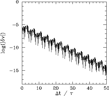
Figure 50 shows the time evolution of the ![]() -component of the phase-space
separation,
-component of the phase-space
separation, ![]() , between two neighbouring trajectories, one of which is the period-8
attractor illustrated in Fig. 46. It can be seen that
, between two neighbouring trajectories, one of which is the period-8
attractor illustrated in Fig. 46. It can be seen that ![]() decays in time,
though not as rapidly as in Fig. 49. Another way of saying this is that the
Liapunov exponent of the periodic attractor shown in Fig. 46
is negative (i.e., it has a negative real part),
though not as negative as that of the periodic attractor shown in Fig. 45.
decays in time,
though not as rapidly as in Fig. 49. Another way of saying this is that the
Liapunov exponent of the periodic attractor shown in Fig. 46
is negative (i.e., it has a negative real part),
though not as negative as that of the periodic attractor shown in Fig. 45.
Figure 51 shows the time evolution of the ![]() -component of the phase-space
separation,
-component of the phase-space
separation, ![]() , between two neighbouring trajectories, one of which is the period-16
attractor illustrated in Fig. 47. It can be seen that
, between two neighbouring trajectories, one of which is the period-16
attractor illustrated in Fig. 47. It can be seen that ![]() decays weakly in
time. In other words, the Liapunov exponent of the periodic attractor shown in Fig. 47 is
small and negative.
decays weakly in
time. In other words, the Liapunov exponent of the periodic attractor shown in Fig. 47 is
small and negative.
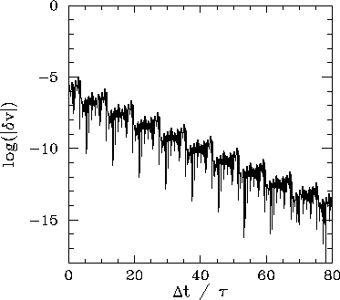
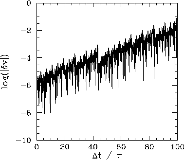
Finally, Fig. 52 shows the time evolution of the ![]() -component of the phase-space
separation,
-component of the phase-space
separation, ![]() , between two neighbouring trajectories, one of which is the chaotic
attractor illustrated in Fig. 48. It can be seen that
, between two neighbouring trajectories, one of which is the chaotic
attractor illustrated in Fig. 48. It can be seen that ![]() increases in
time. In other words, the Liapunov exponent of the chaotic attractor shown in Fig. 48 is
positive. Further investigation reveals that, as the control parameter
increases in
time. In other words, the Liapunov exponent of the chaotic attractor shown in Fig. 48 is
positive. Further investigation reveals that, as the control parameter ![]() is gradually increased, the Liapunov exponent changes sign and becomes positive at exactly the same
point that chaos ensues in Fig 44.
is gradually increased, the Liapunov exponent changes sign and becomes positive at exactly the same
point that chaos ensues in Fig 44.
The above discussion strongly suggests that periodic attractors are characterized by negative Liapunov exponents, whereas chaotic attractors are characterized by positive exponents. But, how can an attractor have a positive Liapunov exponent? Surely, a positive exponent necessarily implies that neighbouring phase-space trajectories diverge from the attractor (and, hence, that the attractor is not a true attractor)? It turns out that this is not the case. The chaotic attractor shown in Fig. 48 is a true attractor, in the sense that neighbouring trajectories rapidly converge onto it--i.e., after a few periods of the external drive their Poincaré sections plot out the same four-line segment shown in Fig. 48. Thus, the exponential divergence of neighbouring trajectories, characteristic of chaotic attractors, takes place within the attractor itself. Obviously, this exponential divergence must come to an end when the phase-space separation of the trajectories becomes comparable to the extent of the attractor.
A dynamical system characterized by a positive Liapunov exponent, ![]() , has a time horizon beyond
which regular deterministic prediction breaks down. Suppose that we measure the initial
conditions of an experimental system very accurately. Obviously, no measurement is perfect: there
is always some error
, has a time horizon beyond
which regular deterministic prediction breaks down. Suppose that we measure the initial
conditions of an experimental system very accurately. Obviously, no measurement is perfect: there
is always some error ![]() between our estimate and the true initial state. After a
time
between our estimate and the true initial state. After a
time ![]() , the discrepancy grows to
, the discrepancy grows to
![]() . Let
. Let ![]() be
a measure of our tolerance: i.e., a prediction within
be
a measure of our tolerance: i.e., a prediction within ![]() of the true state
is
considered acceptable. It follows that our prediction becomes unacceptable when
of the true state
is
considered acceptable. It follows that our prediction becomes unacceptable when
![]() , which occurs when
, which occurs when
| (107) |
It follows, from the above discussion, that chaotic attractors are associated with motion which is essentially unpredictable. In other words, if we attempt to integrate the equations of motion of a chaotic system then even the slightest error made in the initial conditions will be amplified exponentially over time and will rapidly destroy the accuracy of our prediction. Eventually, all that we will be able to say is that the motion lies somewhere on the chaotic attractor in phase-space, but exactly where it lies on the attractor at any given time will be unknown to us.
The hyper-sensitivity of chaotic systems to initial conditions is
sometimes called the butterfly effect. The idea is that a butterfly flapping its wings
in a South American rain-forest could, in principle, affect the weather in Texas (since the atmosphere
exhibits chaotic dynamics). This idea was first publicized by the meteorologist Edward Lorenz,
who constructed a very crude model of the convection of the atmosphere when it is heated from
below by the ground.31 Lorenz discovered, much to his surprise, that his model atmosphere exhibited
chaotic motion--which, at that time, was virtually unknown to physics.
In fact, Lorenz was essentially the first
scientist to fully understand the nature and ramifications of chaotic motion in
physical systems. In particular, Lorenz realized that the chaotic dynamics of the
atmosphere spells the doom of long-term weather forecasting: the best one can hope
to achieve is
to predict the weather a few days in advance (![]() for the atmosphere is of order a
few days).
for the atmosphere is of order a
few days).