Runge-Kutta methods

There are two main reasons why Euler's method is not generally used in scientific computing. Firstly, the truncation error per step associated with this method is far larger than those associated with other, more advanced, methods (for a given value of $h$). Secondly, Euler's method is too prone to numerical instabilities.

The methods most commonly employed by scientists to integrate o.d.e.s were first developed by the German mathematicians C.D.T. Runge and M.W. Kutta in the latter half of the nineteenth century.¹⁴The basic reasoning behind so-called Runge-Kutta methods is outlined in the following.

The main reason that Euler's method has such a large truncation error per step is that in evolving the solution from $x_n$ to $x_{n+1}$ the method only evaluates derivatives at the beginning of the interval: i.e., at $x_n$. The method is, therefore, very asymmetric with respect to the beginning and the end of the interval. We can construct a more symmetric integration method by making an Euler-like trial step to the midpoint of the interval, and then using the values of both $x$ and $y$ at the midpoint to make the real step across the interval. To be more exact,

$$k_1 = h\,f(x_n,y_n),$$ (19)

$$k_2 = h\,f(x_n+h/2, y_n+k_1/2),$$ (20)

$$y_{n+1} = y_n + k_2 + O(h^3).$$ (21)

As indicated in the error term, this symmetrization cancels out the first-order error, making the method second-order. In fact, the above method is generally known as a second-order Runge-Kutta method. Euler's method can be thought of as a first-order Runge-Kutta method.

Of course, there is no need to stop at a second-order method. By using two trial steps per interval, it is possible to cancel out both the first and second-order error terms, and, thereby, construct a third-order Runge-Kutta method. Likewise, three trial steps per interval yield a fourth-order method, and so on.¹⁵

The general expression for the total error, $\epsilon$, associated with integrating our o.d.e. over an $x$-interval of order unity using an $n$th-order Runge-Kutta method is approximately

$$\epsilon \sim \frac{\eta}{h} + h^n.$$ (22)

Here, the first term corresponds to round-off error, whereas the second term represents truncation error. The minimum practical step-length, $h_0$, and the minimum error, $\epsilon _0$, take the values

$$h_0 \sim \eta^{1/(n+1)},$$ (23)

$$\epsilon_0 \sim \eta^{n/(n+1)},$$ (24)

respectively. In Tab. 1, these values are tabulated against $n$ using $\eta = 2.22\times 10^{-16}$ (the value appropriate to double precision arithmetic on IBM-PC clones). It can be seen that $h_0$ increases and $\epsilon _0$ decreases as $n$ gets larger. However, the relative change in these quantities becomes progressively less dramatic as $n$ increases.

Table 1: The minimum practical step-length, $h_0$, and minimum error, $\epsilon _0$, for an $n$th-order Runge-Kutta method integrating over a finite interval using double precision arithmetic on an IBM-PC clone.

$n$	$h_0$	$\epsilon _0$
1	$1.5\times 10^{-8}$	$1.5\times 10^{-8}$
2	$6.1\times 10^{-6}$	$3.7\times 10^{-11}$
3	$1.2\times 10^{-4}$	$1.8\times 10^{-12}$
4	$7.4\times 10^{-4}$	$3.0\times 10^{-13}$
5	$2.4\times 10^{-3}$	$9.0\times 10^{-14}$

In the majority of cases, the limiting factor when numerically integrating an o.d.e. is not round-off error, but rather the computational effort involved in calculating the function $f(x,y)$. Note that, in general, an $n$th-order Runge-Kutta method requires $n$ evaluations of this function per step. It can easily be appreciated that as $n$ is increased a point is quickly reached beyond which any benefits associated with the increased accuracy of a higher order method are more than offset by the computational ``cost'' involved in the necessary additional evaluation of $f(x,y)$ per step. Although there is no hard and fast general rule, in most problems encountered in computational physics this point corresponds to $n=4$. In other words, in most situations of interest a fourth-order Runge Kutta integration method represents an appropriate compromise between the competing requirements of a low truncation error per step and a low computational cost per step.

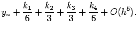
The standard fourth-order Runge-Kutta method takes the form:

$$k_1 = h\,f(x_n,y_n),$$ (25)

$$k_2 = h\,f(x_n+h/2, y_n+k_1/2),$$ (26)

$$k_3 = h\,f(x_n+h/2, y_n+k_2/2),$$ (27)

$$k_4 = h\,f(x_n+h, y_n+k_3),$$ (28)

$$y_{n+1} = y_n + \frac{k_1}{6}+\frac{k_2}{3} +\frac{k_3}{3}+\frac{k_4}{6} +O(h^5).$$ (29)

This is the method which we shall use, throughout this course, to integrate first-order o.d.e.s. The generalization of this method to deal with systems of coupled first-order o.d.e.s is (hopefully) fairly obvious.