


Next: The Ising model
Up: Monte-Carlo methods
Previous: Distribution functions
Consider a one-dimensional integral:
 . We can evaluate this
integral numerically by dividing the interval
. We can evaluate this
integral numerically by dividing the interval  to
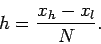
to  into
into  identical subdivisions of
width
identical subdivisions of
width
 |
(326) |
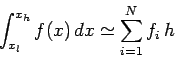
Let  be the midpoint of the
  th subdivision, and let
  .
Our approximation to the integral takes the form
.
Our approximation to the integral takes the form
 |
(327) |
This integration method--which is known as the midpoint method--is not particularly
accurate, but is very easy to generalize to multi-dimensional integrals.
What is the error associated with the midpoint method? Well, the error is the
product of the error per subdivision, which is  , and the number of subdivisions,
which is
, and the number of subdivisions,
which is  . The error per subdivision follows from the linear variation
of
. The error per subdivision follows from the linear variation
of  within each subdivision. Thus, the overall error is
 . Since,
 , we can write
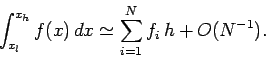 |
(328) |
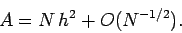
Let us now consider a two-dimensional integral. For instance, the area enclosed by a curve.
We can evaluate such an integral by dividing space into identical squares of dimension  ,
and then counting the number of squares, (say), whose midpoints lie within the curve.
Our approximation to the integral then takes the form
,
and then counting the number of squares, (say), whose midpoints lie within the curve.
Our approximation to the integral then takes the form
 |
(329) |
This is the two-dimensional generalization of the midpoint method.
What is the error associated with the midpoint method in two-dimensions? Well, the error
is generated by those squares which are intersected by the curve. These squares either
contribute wholly or not at all to the integral, depending on whether their midpoints
lie within the curve. In reality, only those parts of the intersected squares which lie
within the curve should contribute to the integral. Thus, the error is the product of
the area of a given square, which is , and the number of squares intersected
by the curve, which is . Hence, the overall error is
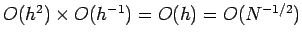 . It follows that we can write
 |
(330) |
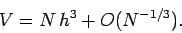
Let us now consider a three-dimensional integral. For instance, the volume enclosed by a surface.
We can evaluate such an integral by dividing space into identical cubes of dimension ,
and then counting the number of cubes, (say), whose midpoints lie within the surface.
Our approximation to the integral then takes the form
 |
(331) |
This is the three-dimensional generalization of the midpoint method.
What is the error associated with the midpoint method in three-dimensions? Well, the error
is generated by those cubes which are intersected by the surface. These cubes either
contribute wholly or not at all to the integral, depending on whether their midpoints
lie within the surface. In reality, only those parts of the intersected cubes which lie
within the surface should contribute to the integral. Thus, the error is the product of
the volume of a given cube, which is  , and the number of cubes intersected
by the surface, which is
, and the number of cubes intersected
by the surface, which is  . Hence, the overall error is
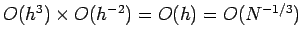 . It follows that we can write
 |
(332) |
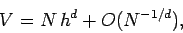
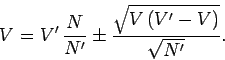
Let us, finally, consider using the midpoint method to evaluate the volume,  , of a
  -dimensional
hypervolume enclosed by a
-dimensional
hypervolume enclosed by a  -dimensional hypersurface. It is clear, from the above examples,
that
-dimensional hypersurface. It is clear, from the above examples,
that
 |
(333) |
where is the number of identical hypercubes into which the hypervolume is divided.
Note the increasingly slow fall-off of the error with as the dimensionality, ,
becomes greater. The explanation for this phenomenon is quite simple. Suppose that  .
With we can divide a unit line into (identical) subdivisions whose linear extent
is
.
With we can divide a unit line into (identical) subdivisions whose linear extent
is  , but we can only divide a unit area into subdivisions whose linear extent
is
, but we can only divide a unit area into subdivisions whose linear extent
is  , and a unit volume into subdivisions whose linear extent
is
, and a unit volume into subdivisions whose linear extent
is  . Thus, for a fixed number of subdivisions the grid spacing (and, hence, the
integration error) increases dramatically
with increasing dimension.
. Thus, for a fixed number of subdivisions the grid spacing (and, hence, the
integration error) increases dramatically
with increasing dimension.
Let us now consider the so-called Monte-Carlo method for evaluating multi-dimensional
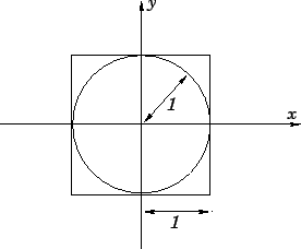
integrals. Consider, for example, the evaluation of the area,  , enclosed by a curve,
  .
Suppose that the curve lies wholly within some simple domain of area
.
Suppose that the curve lies wholly within some simple domain of area  , as
illustrated in Fig. 97. Let us generate
, as
illustrated in Fig. 97. Let us generate  points which are randomly distributed
throughout . Suppose that of these points lie within curve . Our estimate for the area enclosed
by the curve is simply
points which are randomly distributed
throughout . Suppose that of these points lie within curve . Our estimate for the area enclosed
by the curve is simply
 |
(334) |
Figure 97:
The Monte-Carlo integration method.
 |
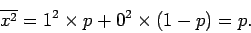
What is the error associated with the Monte-Carlo integration method? Well, each
point has a probability  of lying within the curve. Hence, the determination
of whether a given point lies within the curve is like the measurement of a
random variable
of lying within the curve. Hence, the determination
of whether a given point lies within the curve is like the measurement of a
random variable  which has two possible values: 1 (corresponding to the point being inside the curve)
with probability
which has two possible values: 1 (corresponding to the point being inside the curve)
with probability  , and 0 (corresponding to the point being outside the curve) with probability
 . If we make measurements of (i.e., if we scatter points
throughout ) then the number of points lying within the curve is
. If we make measurements of (i.e., if we scatter points
throughout ) then the number of points lying within the curve is
 |
(335) |
where denotes the th measurement of .
Now, the mean value of is
 |
(336) |
where
 |
(337) |
Hence,
 |
(338) |
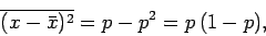
which is consistent with Eq. (334). We conclude that, on average, a measurement of
leads to the correct answer.
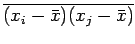
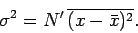
But, what is the scatter in such a measurement? Well, if  represents
the standard deviation of then we have
represents
the standard deviation of then we have
 |
(339) |
which can also be written
 |
(340) |
However,
 equals
 if
if  , and
equals zero, otherwise, since successive measurements of are uncorrelated. Hence,
, and
equals zero, otherwise, since successive measurements of are uncorrelated. Hence,
 |
(341) |
Now,
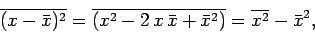 |
(342) |
and
 |
(343) |
Thus,
 |
(344) |
giving
 |
(345) |
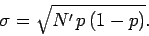
Finally, since the likely values of lie
in the range
 , we can write
 |
(346) |
It follows from Eq. (334) that
 |
(347) |
In other words, the error scales like  .
.
The Monte-Carlo method generalizes immediately to -dimensions.
For instance, consider a -dimensional hypervolume enclosed by a
-dimensional hypersurface . Suppose that lies wholly
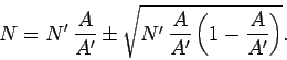
within some simple hypervolume  . We can generate points randomly
distributed throughout . Let be the number of these
points which lie within . It follows that our estimate for
is simply
. We can generate points randomly
distributed throughout . Let be the number of these
points which lie within . It follows that our estimate for
is simply
 |
(348) |
Now, there is nothing in our derivation of Eq. (347) which depends on the
fact that the integral in question is two-dimensional. Hence, we can generalize
this equation to give
 |
(349) |
We conclude that the error associated with Monte-Carlo integration always
scales like , irrespective of the dimensionality of the integral.
We are now in a position to compare and contrast the midpoint and Monte-Carlo
methods for evaluating multi-dimensional integrals.
In the midpoint method, we fill space with an evenly spaced mesh of (say) points
(i.e., the midpoints of the subdivisions), and
the overall error scales like  , where is the dimensionality of the integral.
In the Monte-Carlo method, we fill space with (say) randomly distributed
points, and the overall error scales like
, where is the dimensionality of the integral.
In the Monte-Carlo method, we fill space with (say) randomly distributed
points, and the overall error scales like  , irrespective of the
dimensionality of the integral. For a one-dimensional integral (
, irrespective of the
dimensionality of the integral. For a one-dimensional integral ( ), the
midpoint method is more efficient than the Monte-Carlo method, since in the
former case the error scales like
), the
midpoint method is more efficient than the Monte-Carlo method, since in the
former case the error scales like  , whereas in the latter the
error scales like . For a two-dimensional integral (
, whereas in the latter the
error scales like . For a two-dimensional integral ( ),
the midpoint and Monte-Carlo methods are both equally efficient, since in
both cases the error scales like . Finally, for
a three-dimensional integral (
),
the midpoint and Monte-Carlo methods are both equally efficient, since in
both cases the error scales like . Finally, for
a three-dimensional integral ( ), the
midpoint method is less efficient than the Monte-Carlo method, since in the
former case the error scales like
), the
midpoint method is less efficient than the Monte-Carlo method, since in the
former case the error scales like  , whereas in the latter the
error scales like . We conclude that for a sufficiently high dimension
integral the Monte-Carlo method is always going to be more efficient than an
integration method (such as the midpoint method) which relies on a uniform grid.
, whereas in the latter the
error scales like . We conclude that for a sufficiently high dimension
integral the Monte-Carlo method is always going to be more efficient than an
integration method (such as the midpoint method) which relies on a uniform grid.
Figure 98:
Example calculation: volume of unit-radius 2-dimensional sphere enclosed
in a close-fitting 2-dimensional cube.
 |
Up to now, we have only considered how the Monte-Carlo method can be employed to
evaluate a rather special class of integrals in which the integrand function
can only take the values 0 or 1. However, the Monte-Carlo method can easily be
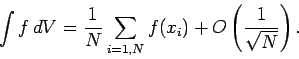
adapted to evaluate more general integrals. Suppose that we
wish to evaluate  , where
  is a general function and the
domain of integration is of arbitrary dimension. We proceed by randomly scattering
points throughout the integration domain and calculating at each point.
Let denote the th point. The Monte-Carlo approximation to the integral
is simply
is a general function and the
domain of integration is of arbitrary dimension. We proceed by randomly scattering
points throughout the integration domain and calculating at each point.
Let denote the th point. The Monte-Carlo approximation to the integral
is simply
 |
(350) |
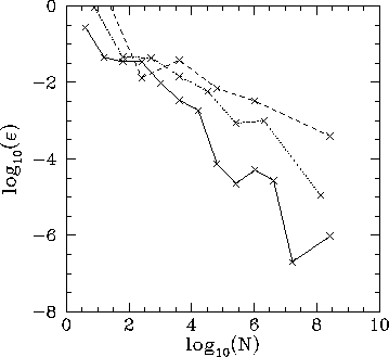
Figure 99:
The integration error,  , versus the number of grid-points, , for three
integrals evaluated using the midpoint method. The integrals are the
area of a unit-radius circle (solid curve), the volume of a unit-radius
sphere (dotted curve), and the volume of a unit-radius 4-sphere (dashed curve).
, versus the number of grid-points, , for three
integrals evaluated using the midpoint method. The integrals are the
area of a unit-radius circle (solid curve), the volume of a unit-radius
sphere (dotted curve), and the volume of a unit-radius 4-sphere (dashed curve).
 |
We end this section with an example calculation. Let us evaluate the volume of a unit-radius -dimensional sphere, where
runs from 2 to 4, using both the midpoint and Monte-Carlo methods. For
both methods, the domain of integration is a cube, centred on the sphere, which is
such that the sphere just touches each face of the cube, as illustrated in Fig. 98.
Figure 100:
The integration error, , versus the number of points, , for three
integrals evaluated using the Monte-Carlo method. The integrals are the
area of a unit-radius circle (solid curve), the volume of a unit-radius
sphere (dotted curve), and the volume of a unit-radius 4-sphere (dashed curve).
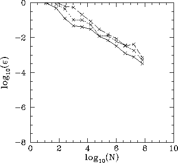 |
Figure 99 shows the integration error associated with the midpoint method
as a function of the number of grid-points, . It can be seen that as the dimensionality
of the integral increases the error falls off much less rapidly as increases.
Figure 100 shows the integration error associated with the Monte-Carlo method
as a function of the number of points, . It can be seen that there is very little
change in the rate at which the error falls off with increasing
as the dimensionality of the integral varies. Hence, as the dimensionality, , increases the Monte-Carlo method
eventually wins out over the midpoint method.
Next: The Ising model
Up: Monte-Carlo methods
Previous: Distribution functions
Richard Fitzpatrick
2006-03-29