The most well-known algorithm for generating psuedo-random sequences
of integers is the so-called linear congruental method.
The formula linking the ![]() th and
th and ![]() th integers in the sequence is
th integers in the sequence is
Consider an example case in which ![]() ,
, ![]() , and
, and ![]() . A typical sequence of numbers generated by
formula (312) is
. A typical sequence of numbers generated by
formula (312) is
| (313) |
The function listed below is an implementation of the linear congruental method.
// random.cpp

// Linear congruential psuedo-random number generator.
// Generates psuedo-random sequence of integers in
//  range 0 .. RANDMAX.

#define RANDMAX 6074  // RANDMAX = M - 1

int random (int seed = 0)
{
  static int next = 1;
  static int A = 106;
  static int C = 1283;
  static int M = 6075;

  if (seed) next = seed;
  next = next * A + C;
  return next % M;
}
The keyword static in front of a local variable declaration indicates that the
program should preserve the value of
that variable between function calls. In other words, if the static variable next
has the value 999 on exit from function random then the next time this function is
called next will have exactly the same value. Note that the values of non-static
local variables are not preserved between function calls. The = 0 in the first line
of function random is a default value for the argument seed. In fact, random
can be called in one of two ways. Firstly, random can be called with no argument: i.e.,
random (): in which case, seed is given the default value 0. Secondly, random
can be called with an integer argument: i.e.,
random (n): in which case, the value of seed is set to n. The first way of calling
random just returns the next integer in the psuedo-random sequence. The
second way seeds the sequence with the value n (i.e.,
The above function returns a pseudo-random integer in the range ![]() to RANDMAX (where RANDMAX
takes the value
to RANDMAX (where RANDMAX
takes the value ![]() ). In order to obtain a random variable
). In order to obtain a random variable ![]() , uniformly distributed in the
range 0 to 1, we would write
, uniformly distributed in the
range 0 to 1, we would write
x = double (random ()) / double (RANDMAX);Now if
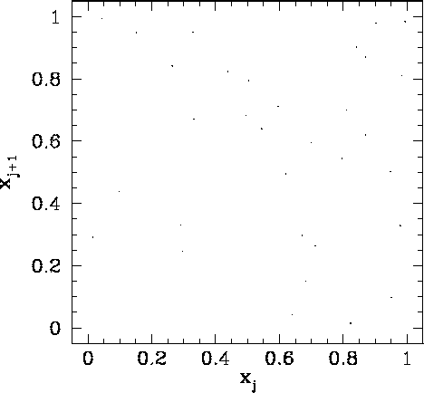 |
Figure 91 shows a correlation plot for the first 10000 ![]() -
-![]() pairs generated
using a linear congruental psuedo-random number generator characterized by
pairs generated
using a linear congruental psuedo-random number generator characterized by
![]() ,
, ![]() , and
, and ![]() . It can be seen that this is a
poor choice of values for
. It can be seen that this is a
poor choice of values for
![]() ,
, ![]() , and
, and ![]() , since the pseudo-random sequence repeats after a few iterations, yielding
, since the pseudo-random sequence repeats after a few iterations, yielding
![]() values which do not densely fill the interval 0 to 1.
values which do not densely fill the interval 0 to 1.
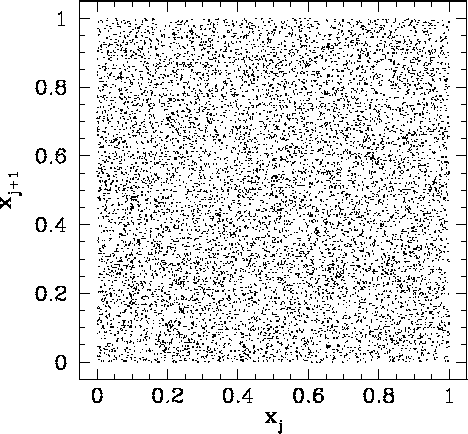 |
Figure 92 shows a correlation plot for the first 10000 ![]() -
-![]() pairs generated
using a linear congruental psuedo-random number generator characterized by
pairs generated
using a linear congruental psuedo-random number generator characterized by
![]() ,
, ![]() , and
, and ![]() . It can be seen that this is a
far better choice of values for
. It can be seen that this is a
far better choice of values for
![]() ,
, ![]() , and
, and ![]() , since the pseudo-random sequence is of maximal length, yielding
, since the pseudo-random sequence is of maximal length, yielding
![]() values which are fairly evenly distributed in the range 0 to 1. However,
if we look carefully at Fig. 92, we can see that there is a slight tendency for
the dots to line up in the horizontal and vertical directions. This indicates that the
values which are fairly evenly distributed in the range 0 to 1. However,
if we look carefully at Fig. 92, we can see that there is a slight tendency for
the dots to line up in the horizontal and vertical directions. This indicates that the
![]() are not quite randomly distributed: i.e., there is some correlation between
successive
are not quite randomly distributed: i.e., there is some correlation between
successive ![]() values. The problem is that
values. The problem is that ![]() is too low: i.e., there is
not a sufficiently wide selection of different
is too low: i.e., there is
not a sufficiently wide selection of different ![]() values in the interval 0 to 1.
values in the interval 0 to 1.
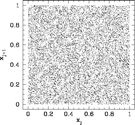 |
Figure 93 shows a correlation plot for the first 10000 ![]() -
-![]() pairs generated
using a linear congruental psuedo-random number generator characterized by
pairs generated
using a linear congruental psuedo-random number generator characterized by
![]() ,
, ![]() , and
, and ![]() . The clumping of points in this figure indicates
that the
. The clumping of points in this figure indicates
that the ![]() are again not quite randomly distributed. This time the problem is integer overflow:
i.e., the values of
are again not quite randomly distributed. This time the problem is integer overflow:
i.e., the values of ![]() and
and ![]() are sufficiently large that
are sufficiently large that
![]() for
many integers in the pseudo-random sequence. Thus, the algorithm (312) is not
being executed correctly.
for
many integers in the pseudo-random sequence. Thus, the algorithm (312) is not
being executed correctly.
Integer overflow can be overcome using Schrange's algorithm. If
![]() then
then
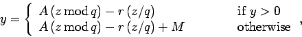 |
(314) |
// random.cpp

// Park and Miller's psuedo-random number generator.

#define RANDMAX 2147483646 // RANDMAX = M - 1

int random (int seed = 0)
{
  static int next = 1;
  static int A = 16807;
  static int M = 2147483647;   // 2^31 - 1
  static int q = 127773;       // M / A
  static int r = 2836;         // M % A

  if (seed) next = seed;
  next = A * (next % q) - r * (next / q);
  if (next < 0) next += M;
  return next;
}
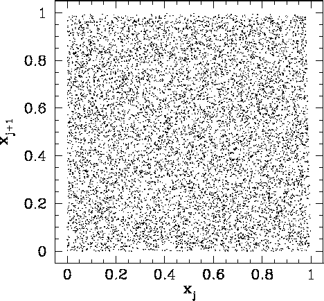 |
Figure 94 shows a correlation plot for the first 10000 ![]() -
-![]() pairs generated
using Park & Miller's method.
We can now see no pattern whatsoever in the plotted points. This indicates that the
pairs generated
using Park & Miller's method.
We can now see no pattern whatsoever in the plotted points. This indicates that the ![]() are indeed
randomly distributed in the range 0 to 1. From now on, we shall use Park & Miller's method
to generate all the psuedo-random numbers needed in our investigation of Monte-Carlo methods.
are indeed
randomly distributed in the range 0 to 1. From now on, we shall use Park & Miller's method
to generate all the psuedo-random numbers needed in our investigation of Monte-Carlo methods.