Simple Harmonic Oscillator Equation
Suppose that a physical system possessing a single degree of freedom—that is, a
system whose instantaneous state at time  is fully described by a single dependent variable,
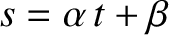
  —obeys the following time evolution equation [cf., Equation (1.2)],
 |
(1.17) |
where  is a constant. As we have seen, this differential
equation is called the simple harmonic oscillator equation, and has the
standard solution
is a constant. As we have seen, this differential
equation is called the simple harmonic oscillator equation, and has the
standard solution
 |
(1.18) |
where  and
and  are constants. Moreover, this solution describes a type of oscillation
characterized by a constant amplitude,
are constants. Moreover, this solution describes a type of oscillation
characterized by a constant amplitude,  , and a constant angular frequency,
  .
The phase angle, , determines the times at which the oscillation attains its
maximum value. The frequency of the oscillation (in hertz) is
.
The phase angle, , determines the times at which the oscillation attains its
maximum value. The frequency of the oscillation (in hertz) is
 ,
and the period is
,
and the period is
 . The frequency and period of the
oscillation are both determined by the constant , which appears in the simple harmonic oscillator equation, whereas the amplitude, , and phase angle, , are determined by the initial conditions. [See Equations (1.10)–(1.13).] In fact, and are the two arbitrary constants of integration of the
second-order ordinary differential equation (1.17). Recall, from standard differential equation theory (Riley 1974), that the
most general solution of an
. The frequency and period of the
oscillation are both determined by the constant , which appears in the simple harmonic oscillator equation, whereas the amplitude, , and phase angle, , are determined by the initial conditions. [See Equations (1.10)–(1.13).] In fact, and are the two arbitrary constants of integration of the
second-order ordinary differential equation (1.17). Recall, from standard differential equation theory (Riley 1974), that the
most general solution of an  th-order ordinary differential equation (i.e.,
an equation involving a single independent variable, and a single dependent variable, in which the highest derivative of the dependent with respect to the
independent variable is
th-order, and the lowest zeroth-order) involves arbitrary constants of integration. (Essentially, this is because
we have to integrate the equation times with respect to the independent variable to reduce it to zeroth-order, and so
obtain the solution. Furthermore, each integration introduces an arbitrary constant. For example,
the integral of
th-order ordinary differential equation (i.e.,
an equation involving a single independent variable, and a single dependent variable, in which the highest derivative of the dependent with respect to the
independent variable is
th-order, and the lowest zeroth-order) involves arbitrary constants of integration. (Essentially, this is because
we have to integrate the equation times with respect to the independent variable to reduce it to zeroth-order, and so
obtain the solution. Furthermore, each integration introduces an arbitrary constant. For example,
the integral of
 , where
  is a known constant, is
 , where
  is an arbitrary constant.)
Multiplying Equation (1.17) by  , we obtain
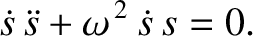 |
(1.19) |
However, this can also be written
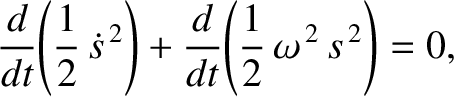 |
(1.20) |
or
 |
(1.21) |
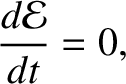
where
 |
(1.22) |
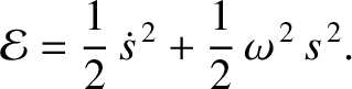
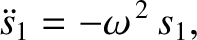
According to Equation (1.21),  is a conserved quantity. In other words, it does not vary with time. This quantity is
generally proportional to the overall energy of the system. For instance, would be the energy divided by the mass in
the mass–spring system discussed in Section 1.2. The quantity is either
zero or positive, because neither of the terms on the right-hand side of Equation (1.22) can be negative.
is a conserved quantity. In other words, it does not vary with time. This quantity is
generally proportional to the overall energy of the system. For instance, would be the energy divided by the mass in
the mass–spring system discussed in Section 1.2. The quantity is either
zero or positive, because neither of the terms on the right-hand side of Equation (1.22) can be negative.
Let us search for an equilibrium state. Such a state is
characterized by
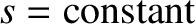 , so that
 . It follows
from Equation (1.17) that
. It follows
from Equation (1.17) that  , and from Equation (1.22) that
 . We conclude that the system can only remain permanently at
rest when
.
Conversely, the system can
never permanently come to rest when
. We conclude that the system can only remain permanently at
rest when
.
Conversely, the system can
never permanently come to rest when
 , and must, therefore, keep moving for ever. Because the equilibrium state is characterized by , we deduce that
 represents a kind of “displacement” of the system from this state.
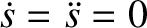
It is also apparent, from Equation (1.22), that attains its maximum value when
represents a kind of “displacement” of the system from this state.
It is also apparent, from Equation (1.22), that attains its maximum value when  .
In fact,
.
In fact,
 |
(1.23) |
where
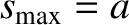 is the amplitude of the oscillation.
Likewise, attains its maximum value,
is the amplitude of the oscillation.
Likewise, attains its maximum value,
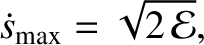 |
(1.24) |
when .
The simple harmonic oscillation specified by Equation (1.18) can also
be written in the form
 |
(1.25) |
where
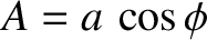 and
and
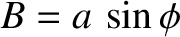 . Here, we have employed the trigonometric identity
 . (See Appendix B.)
Alternatively, Equation (1.18) can be written
. (See Appendix B.)
Alternatively, Equation (1.18) can be written
 |
(1.26) |
where
 , and use has been made of the trigonometric
identity
, and use has been made of the trigonometric
identity
 . (See Appendix B.) It follows that there are many different
ways of representing a simple harmonic oscillation, but they all involve
linear combinations of sine and cosine functions whose arguments
take the form
. (See Appendix B.) It follows that there are many different
ways of representing a simple harmonic oscillation, but they all involve
linear combinations of sine and cosine functions whose arguments
take the form
 , where
  is some constant. However,
irrespective of its form,
a general solution to the simple harmonic oscillator equation must always contain two arbitrary constants. For example,
is some constant. However,
irrespective of its form,
a general solution to the simple harmonic oscillator equation must always contain two arbitrary constants. For example,  and
and  in Equation (1.25), or
and
in Equation (1.25), or
and  in Equation (1.26).
The simple harmonic oscillator equation, (1.17), is a linear differential equation,
which means that
if is a solution then so is  , where is
an arbitrary constant. This can be verified by multiplying the equation by ,
and then making use of the fact that
, where is
an arbitrary constant. This can be verified by multiplying the equation by ,
and then making use of the fact that
 . Linear
differential equations have the very important and useful property that their
solutions are superposable. This means that if
. Linear
differential equations have the very important and useful property that their
solutions are superposable. This means that if  is a
solution to Equation (1.17), so
that
is a
solution to Equation (1.17), so
that
 |
(1.27) |
and
 is a different solution, so that
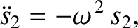 |
(1.28) |
then
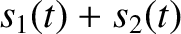 is also a solution. This can be verified by adding the previous
two equations, and making use of the fact that
is also a solution. This can be verified by adding the previous
two equations, and making use of the fact that
 . Furthermore, it can be demonstrated that any linear combination of
  and
and  ,
such as
,
such as
 , where and are arbitrary constants, is also a solution.
It is very helpful to know this fact.
For instance, the special solution to the simple harmonic oscillator equation, (1.17), with the simple initial
conditions
, where and are arbitrary constants, is also a solution.
It is very helpful to know this fact.
For instance, the special solution to the simple harmonic oscillator equation, (1.17), with the simple initial
conditions  and
and
 can easily be shown to be
 |
(1.29) |
Likewise, the special solution with the simple initial conditions  and
and
 is
is
 |
(1.30) |
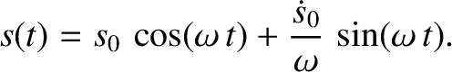
Thus, because the solutions to the simple harmonic oscillator equation are superposable, the
solution with the general initial conditions  and
and
 becomes
 |
(1.31) |
or
 |
(1.32) |