Next: Dirac Delta Function Up: Wave Pulses Previous: Introduction Contents
 that is periodic in
  with period
  . In other
words,
for all . Recall, from Section 5.5, that we can
represent such a function as a Fourier series; that is,
where
. In other
words,
for all . Recall, from Section 5.5, that we can
represent such a function as a Fourier series; that is,
where
 |
(8.3) |
 term in Equation (8.2), for the sake of convenience.]
Equation (8.2) automatically satisfies the periodicity constraint (8.1), because
term in Equation (8.2), for the sake of convenience.]
Equation (8.2) automatically satisfies the periodicity constraint (8.1), because
 and
and
 for all
  and
and  (with the proviso that is an integer).
The so-called Fourier coefficients,
(with the proviso that is an integer).
The so-called Fourier coefficients,  and
and  , appearing in Equation (8.2), can
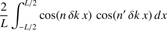
be determined from the function by means of the following readily demonstrated (see Exercise 1)
results:
where ,
, appearing in Equation (8.2), can
be determined from the function by means of the following readily demonstrated (see Exercise 1)
results:
where ,  are positive integers. Here,
 is a Kronecker delta function.
In fact,
(See Exercise 1.)
Incidentally, any periodic function of can be represented as a
Fourier series.
is a Kronecker delta function.
In fact,
(See Exercise 1.)
Incidentally, any periodic function of can be represented as a
Fourier series.
Suppose, however, that we are dealing with a function that is not periodic in .
We can think of such a function as one that is periodic in with a period that
tends to infinity. Does this mean that we can still represent as a Fourier series?
Consider what happens to the series (8.2) in the limit
 , or, equivalently,
 . The series is basically a weighted sum of sinusoidal functions
whose wavenumbers take the quantized values
. The series is basically a weighted sum of sinusoidal functions
whose wavenumbers take the quantized values
 . Moreover, as
, these values become more and more closely
spaced. In fact, we can write
. Moreover, as
, these values become more and more closely
spaced. In fact, we can write
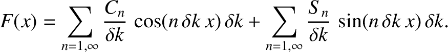
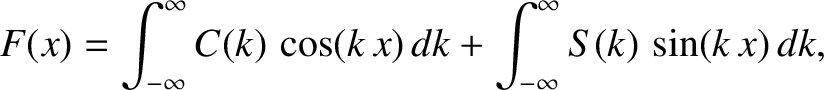
, the summations in the previous expression become integrals, and
we obtain
where
 ,
,
 , and
, and
 .
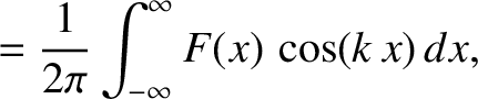
Thus, for the case of an aperiodic function, the Fourier series (8.2) morphs into the so-called Fourier transform (8.10). This transform can be inverted using the continuum limits (i.e., the limit
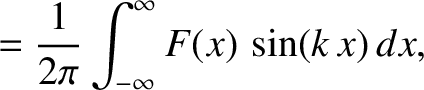
) of Equations (8.7) and (8.8), which are readily shown to be
respectively. (See Exercise 5.)
The previous equations confirm that
.
Thus, for the case of an aperiodic function, the Fourier series (8.2) morphs into the so-called Fourier transform (8.10). This transform can be inverted using the continuum limits (i.e., the limit
) of Equations (8.7) and (8.8), which are readily shown to be
respectively. (See Exercise 5.)
The previous equations confirm that
 and
and
 .
The Fourier-space (i.e.,
.
The Fourier-space (i.e.,  -space) functions
  and
and  are known as the cosine Fourier transform and
the sine Fourier transform of the real-space (i.e., -space) function , respectively.
Furthermore, because we already know that any periodic function can be represented as a Fourier series, it seems
plausible that any aperiodic function can be represented as a Fourier transform. This is indeed the case.
are known as the cosine Fourier transform and
the sine Fourier transform of the real-space (i.e., -space) function , respectively.
Furthermore, because we already know that any periodic function can be represented as a Fourier series, it seems
plausible that any aperiodic function can be represented as a Fourier transform. This is indeed the case.
When sinusoidal waves of different amplitudes, phases, and wavelengths are superposed, they interfere with one another. In some regions of space, the interference is constructive, and the resulting wave amplitude is comparatively large. In other regions, the interference is destructive, and the resulting wave amplitude is comparatively small, or even zero. Equations (8.10)–(8.12) essentially allow us to construct an interference pattern that mimics any given function of position (in one dimension). Alternatively, they allow us to decompose any given function of position into sinusoidal waves that, when superposed, reconstruct the function. Let us consider some examples.
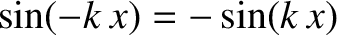
Consider the “top-hat” function,
See Figure 8.1. Given that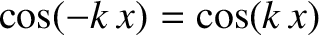 and
and
 , it follows from Equations (8.11) and (8.12) that if is even in , so that
 , then
  , and
if is odd in , so that
, and
if is odd in , so that
 , then
  . Hence, because the top-hat function (8.13)
is even in , its sine Fourier transform is automatically zero. On the other hand,
its cosine Fourier transform takes the form
. Hence, because the top-hat function (8.13)
is even in , its sine Fourier transform is automatically zero. On the other hand,
its cosine Fourier transform takes the form
 |
(8.14) |
, together with its associated cosine transform, .
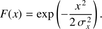
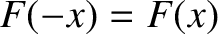
As a second example, consider the so-called Gaussian function,
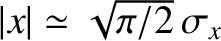
As illustrated in Figure 8.2, this is a smoothly-varying even function of that attains
its peak value  at
at  , and becomes completely negligible when
 . Thus,
  is a measure of the “width” of the function in real (as opposed to Fourier) space.
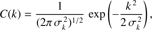
By symmetry, the sine Fourier transform of the preceding function is zero. On the
other hand, the cosine Fourier transform is readily shown to be
where
is a measure of the “width” of the function in real (as opposed to Fourier) space.
By symmetry, the sine Fourier transform of the preceding function is zero. On the
other hand, the cosine Fourier transform is readily shown to be
where
 |
(8.17) |
 .
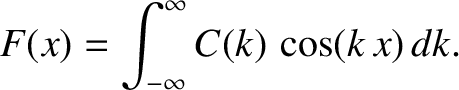
The original function can be reconstructed from
its Fourier transform using
This reconstruction is simply a linear superposition of cosine waves of differing wavenumbers. Moreover, can be interpreted as the amplitude of waves of wavenumber within this superposition. The fact that is a Gaussian of
characteristic width
[which means that is negligible for
.
The original function can be reconstructed from
its Fourier transform using
This reconstruction is simply a linear superposition of cosine waves of differing wavenumbers. Moreover, can be interpreted as the amplitude of waves of wavenumber within this superposition. The fact that is a Gaussian of
characteristic width
[which means that is negligible for
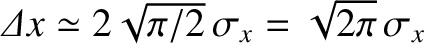
 ] implies that in order to reconstruct a real-space function whose
width in real space is approximately it is necessary to combine sinusoidal functions
with a range of different wavenumbers that is approximately
in extent. To be slightly more exact, the real-space Gaussian function falls to
half of its peak value when
] implies that in order to reconstruct a real-space function whose
width in real space is approximately it is necessary to combine sinusoidal functions
with a range of different wavenumbers that is approximately
in extent. To be slightly more exact, the real-space Gaussian function falls to
half of its peak value when
 . Hence, the full width at half maximum of the function is
 . Likewise, the full width at half maximum of the Fourier-space Gaussian function is
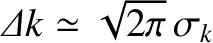 .
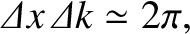
Thus,
.
Thus,
 |
(8.19) |
 .
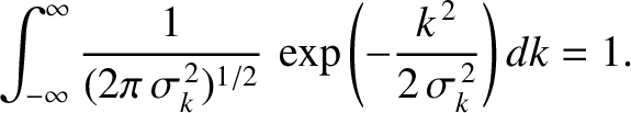
We conclude that a function that is highly localized in real space has a transform that is
highly delocalized in Fourier space, and vice versa. Finally,
(See Exercise 3.)
In other words, a Gaussian function in real space, of unit height and characteristic width , has a cosine Fourier transform
that is a Gaussian in Fourier space, of characteristic width
, and whose integral over all
-space is unity.
.
We conclude that a function that is highly localized in real space has a transform that is
highly delocalized in Fourier space, and vice versa. Finally,
(See Exercise 3.)
In other words, a Gaussian function in real space, of unit height and characteristic width , has a cosine Fourier transform
that is a Gaussian in Fourier space, of characteristic width
, and whose integral over all
-space is unity.
![$\displaystyle F(x)= \sum_{n=1,\infty} \left[C_n\,\cos(n\,\delta k\,x) + S_n\,\sin(n\,\delta k\,x)\right],$](img2323.png)


![\includegraphics[width=1\textwidth]{Chapter08/fig8_01.eps}](img2349.png)
![\includegraphics[width=0.8\textwidth]{Chapter08/fig8_02.eps}](img2358.png)