Next: Simple Harmonic Oscillator Equation Up: Simple Harmonic Oscillation Previous: Introduction Contents
 that slides over a frictionless horizontal surface. Suppose that
the mass is attached
to one end of a light horizontal spring whose other end is anchored in an immovable wall. See
Figure 1.1. At time
that slides over a frictionless horizontal surface. Suppose that
the mass is attached
to one end of a light horizontal spring whose other end is anchored in an immovable wall. See
Figure 1.1. At time  , let
, let  be the extension of the spring; that is, the difference between
the spring's actual length and its unstretched length. can also be used as
a coordinate to determine the instantaneous horizontal displacement of the mass.
be the extension of the spring; that is, the difference between
the spring's actual length and its unstretched length. can also be used as
a coordinate to determine the instantaneous horizontal displacement of the mass.
The equilibrium state of the system corresponds to the situation in which
the mass is at rest, and the spring is unextended (i.e.,
 , where
 ).
In this state, zero horizontal force acts on the mass, and so there is no reason for it to start to move.
However, if the system is perturbed from its equilibrium state (i.e., if the mass is displaced horizontally, such that the
spring becomes extended) then the mass experiences a horizontal force given by Hooke's law,
).
In this state, zero horizontal force acts on the mass, and so there is no reason for it to start to move.
However, if the system is perturbed from its equilibrium state (i.e., if the mass is displaced horizontally, such that the
spring becomes extended) then the mass experiences a horizontal force given by Hooke's law,
 is the so-called force constant of the spring. The negative sign in the preceding expression indicates that
  is a so-called restoring force that always
acts to return the displacement,
is a so-called restoring force that always
acts to return the displacement,  , to its equilibrium value,
  (i.e., if the displacement is
positive then the force is negative, and vice versa).
Note that the magnitude of the restoring
force is directly proportional to the displacement of the mass from its equilibrium
position
(i.e.,
(i.e., if the displacement is
positive then the force is negative, and vice versa).
Note that the magnitude of the restoring
force is directly proportional to the displacement of the mass from its equilibrium
position
(i.e.,
 ). Hooke's law only holds for relatively small spring extensions.
Hence, the mass's displacement cannot be made too large, otherwise Equation (1.1) ceases to be valid.
Incidentally, the motion of this particular dynamical system is representative of the
motion of a wide variety of different mechanical systems when they are slightly disturbed from a stable equilibrium state. (See Sections 1.5 and 1.6.)
). Hooke's law only holds for relatively small spring extensions.
Hence, the mass's displacement cannot be made too large, otherwise Equation (1.1) ceases to be valid.
Incidentally, the motion of this particular dynamical system is representative of the
motion of a wide variety of different mechanical systems when they are slightly disturbed from a stable equilibrium state. (See Sections 1.5 and 1.6.)
Newton's second law of motion leads to the following time evolution equation for the system (Fitzpatrick 2012),
where .
This differential equation is known as the simple harmonic oscillator equation, and its solution has been known
for centuries. The solution can be written
where
.
This differential equation is known as the simple harmonic oscillator equation, and its solution has been known
for centuries. The solution can be written
where  ,
,  , and
, and  are constants. We can demonstrate that Equation (1.3) is indeed a
solution of Equation (1.2) by direct substitution. Plugging the right-hand side of Equation (1.3) into
Equation (1.2), and recalling from standard calculus that
are constants. We can demonstrate that Equation (1.3) is indeed a
solution of Equation (1.2) by direct substitution. Plugging the right-hand side of Equation (1.3) into
Equation (1.2), and recalling from standard calculus that
 and
and
 (see Appendix B), so that
 and
and
 , where use has been made of
the chain rule (Riley 1974),
, where use has been made of
the chain rule (Riley 1974),
![$\displaystyle \frac{d}{dx}\left(f\left[g(x)\right]\right)\equiv \frac{df}{dg}\,\frac{dg}{dx},$](img155.png) |
(1.4) |
 |
(1.5) |
Figure 1.2 shows a graph of versus derived from Equation (1.3). The type of motion displayed here is
called simple harmonic oscillation.
It can be seen that
the displacement oscillates between  and
and  . This result can be obtained from Equation (1.3) by noting that
 . Here,
  is termed the amplitude
of the oscillation. Moreover, the motion is repetitive in time (i.e., it repeats exactly after
a certain time period has elapsed). The repetition period is
is termed the amplitude
of the oscillation. Moreover, the motion is repetitive in time (i.e., it repeats exactly after
a certain time period has elapsed). The repetition period is
 |
(1.7) |
 is a periodic function
of
is a periodic function
of  with
period
with
period  ; that is,
 . It follows that
the motion repeats each time
. It follows that
the motion repeats each time  increases by . In other words, each time increases by
 .
The frequency of the motion (i.e., the number of oscillations completed per
second) is
.
The frequency of the motion (i.e., the number of oscillations completed per
second) is
 |
(1.8) |
 is the motion's angular frequency; that is, the frequency
 converted into radians per second. (The units of are hertz—otherwise
known as cycles per second—whereas the units of are radians per second. One cycle per second is equivalent to radians per second.)
Finally, the phase angle, , determines the times at which the oscillation attains its maximum displacement,
converted into radians per second. (The units of are hertz—otherwise
known as cycles per second—whereas the units of are radians per second. One cycle per second is equivalent to radians per second.)
Finally, the phase angle, , determines the times at which the oscillation attains its maximum displacement,
 . In fact, because the maxima of
occur at
. In fact, because the maxima of
occur at
 , where
 is an arbitrary integer, the times of maximum displacement are
 |
(1.9) |
![\includegraphics[width=0.8\textwidth]{Chapter01/fig1_03.eps}](img176.png) |
Table 1.1 lists the displacement, velocity, and acceleration of the mass at various key points on the simple harmonic oscillation cycle. The information contained in this table is derived from Equation (1.3). All of the non-zero values shown in the table represent either the maximum or the minimum value taken by the quantity in question during the oscillation cycle. The variation of the displacement, velocity, and acceleration during the oscillation cycle is illustrated in Figure 1.4.
![\includegraphics[width=0.75\textwidth]{Chapter01/fig1_04.eps}](img187.png) |
As we have seen, when a mass on a spring is disturbed it executes simple harmonic
oscillation about its equilibrium position. In physical terms, if the mass's initial displacement is positive ( ) then the
force is negative, and pulls the mass toward the equilibrium point (). However,
when the mass reaches this point it is moving, and its inertia thus carries it onward,
so that it acquires a negative displacement (
) then the
force is negative, and pulls the mass toward the equilibrium point (). However,
when the mass reaches this point it is moving, and its inertia thus carries it onward,
so that it acquires a negative displacement ( ). The force then becomes positive, and pulls the mass toward the equilibrium point. However, inertia again carries it past this point, and the mass acquires a positive displacement.
The motion subsequently repeats itself ad infinitum.
). The force then becomes positive, and pulls the mass toward the equilibrium point. However, inertia again carries it past this point, and the mass acquires a positive displacement.
The motion subsequently repeats itself ad infinitum.
The standard solution, (1.3), of the simple harmonic oscillator equation, (1.2), contains three constants: the angular frequency ; the
amplitude, ; and the phase angle, .
The angular frequency is determined by the spring constant,
; the
amplitude, ; and the phase angle, .
The angular frequency is determined by the spring constant,  , and the system
inertia, , via Equation (1.6). It follows that is determined by the
simple harmonic oscillator equation itself (because both and explicitly
appear in this equation).
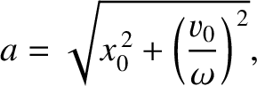
On the other hand, the amplitude and phase angle are determined by the initial conditions.
To be more exact, suppose that the instantaneous displacement and velocity of the mass at
, and the system
inertia, , via Equation (1.6). It follows that is determined by the
simple harmonic oscillator equation itself (because both and explicitly
appear in this equation).
On the other hand, the amplitude and phase angle are determined by the initial conditions.
To be more exact, suppose that the instantaneous displacement and velocity of the mass at  are
are  and
and  ,
respectively. It follows from Equation (1.3) that
,
respectively. It follows from Equation (1.3) that
 |
 |
(1.10) |
 |
 |
(1.11) |
 and
and
 . (See Appendix B.) Hence, we deduce that
 |
(1.12) |
 and
and
 . (See Appendix B.)
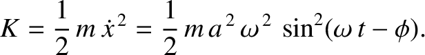
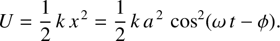
The kinetic energy of the system, which is the same as the kinetic energy of the mass, is written
 |
(1.14) |
 |
(1.15) |
 and
. According to the previous expression, the
total energy is a constant of the motion, and is proportional to the amplitude squared of the oscillation.
Hence, we deduce that the simple harmonic oscillation of a
mass on a spring is characterized
by a continual back and forth flow of energy between kinetic and potential components.
The kinetic energy attains its maximum value, and the potential energy its minimum value, when the displacement is zero (i.e., when ). Likewise,
the potential energy attains its maximum value, and the kinetic energy
its minimum value, when the displacement is maximal (i.e., when
and
. According to the previous expression, the
total energy is a constant of the motion, and is proportional to the amplitude squared of the oscillation.
Hence, we deduce that the simple harmonic oscillation of a
mass on a spring is characterized
by a continual back and forth flow of energy between kinetic and potential components.
The kinetic energy attains its maximum value, and the potential energy its minimum value, when the displacement is zero (i.e., when ). Likewise,
the potential energy attains its maximum value, and the kinetic energy
its minimum value, when the displacement is maximal (i.e., when  ).
The minimum value of
).
The minimum value of  is zero, because the system is instantaneously at rest
when the displacement is maximal. The time variation of the kinetic, potential, and total
energy of a mass on a spring is illustrated in Figure 1.5.
is zero, because the system is instantaneously at rest
when the displacement is maximal. The time variation of the kinetic, potential, and total
energy of a mass on a spring is illustrated in Figure 1.5.
![\includegraphics[width=0.75\textwidth]{Chapter01/fig1_05.eps}](img211.png) |
![\includegraphics[width=0.7\textwidth]{Chapter01/fig1_01.eps}](img137.png)
![\includegraphics[width=0.8\textwidth]{Chapter01/fig1_02.eps}](img158.png)


![$[K(t)+U(t)]/E$](img11.png)