Two Coupled LC Circuits

Consider the LC circuit pictured in Figure 3.4. Let $I_1(t)$, $I_2(t)$, and $I_3(t)$ be the currents flowing in the three legs of the circuit, which meet at junctions $A$ and $B$. According to Kirchhoff's first circuital law, the net current flowing into each junction is zero (Grant and Phillips 1975). It follows that $I_3=-(I_1+I_2)$. We deduce that this is a two-degree-of-freedom system whose instantaneous configuration is specified by the two independent variables $I_1(t)$ and $I_2(t)$. It follows that there are two independent normal modes of oscillation. The potential drops across the left, middle, and right legs of the circuit are $Q_1/C+L\,\dot{I}_1$, $Q_3/C'$, and $Q_2/C+L\,\dot{I}_2$, respectively, where $\dot{Q}_1=I_1$, $\dot{Q}_2=I_2$, and $Q_3=-(Q_1+Q_2)$. However, because the three legs are connected in parallel with one another, the potential drops must all be equal, so that

$$Q_1/C + L\,\dot{I}_1 = Q_3/C' = -(Q_1+Q_2)/C',$$ (3.34)

$$Q_2/C+L\,\dot{I}_2 = Q_3/C' = -(Q_1+Q_2)/C'.$$ (3.35)

Differentiating with respect to $t$, dividing by $L$, and rearranging, we obtain the coupled time evolution equations of the system:

$$\ddot{I}_1 + \omega_0^{\,2}\,(1+\alpha)\,I_1+\omega_0^{\,2}\, \alpha\,I_2 =0,$$ (3.36)

$$\ddot{I}_2 + \omega_0^{\,2}\,(1+\alpha)\,I_2+ \omega_0^{\,2}\,\alpha\,I_1 =0,$$ (3.37)

where $\omega_0=1/\sqrt{L\,C}$ and $\alpha=C/C'$.

Figure 3.4: A two-degree-of-freedom LC circuit.

We can solve the problem in a systematic manner by searching for a normal mode of the form

$$I_1(t) =\hat{I}_1\,\cos(\omega\,t-\phi),$$ (3.38)

$$I_2(t) =\hat{I}_2\,\cos(\omega\,t-\phi).$$ (3.39)

Substitution into the time evolution equations (3.36) and (3.37) yields the homogeneous matrix equation

$$\left( \begin{array}{cc} \hat{\omega}^{\,2}-(1+\alpha), & -\a... ...ht) = \left( \begin{array}{c} 0\\ [0.5ex] 0 \end{array}\right),$$ (3.40)

where $\hat{\omega}=\omega/\omega_0$. The normal frequencies are determined by setting the determinant of the matrix to zero. This gives

$$\left[\hat{\omega}^{\,2}-(1+\alpha)\right]^{\,2}-\alpha^{\,2} = 0,$$ (3.41)

or

$$\hat{\omega}^{\,4} - 2\,(1+\alpha)\,\hat{\omega}^{\,2}+1+2\,\alph... ...eft(\hat{\omega}^{\,2}-1\right)\left(\hat{\omega}^{\,2}-[1+2\,\alpha]\right)=0.$$ (3.42)

The roots of the preceding equation are $\hat{\omega}=1$ and $\hat{\omega}=(1+2\,\alpha)^{1/2}$. (Again, we have neglected the negative frequency roots, because they generate the same patterns of motion as the corresponding positive frequency roots.) Hence, the two normal frequencies are $\omega_0$ and $(1+2\,\alpha)^{1/2}\,\omega_0$. The characteristic patterns of motion associated with the normal modes can be calculated from the first row of the matrix equation (3.40), which can be rearranged to give

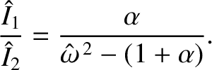$$\frac{\hat{I}_1}{\hat{I}_2}= \frac{\alpha}{\hat{\omega}^{\,2}-(1+\alpha)}.$$ (3.43)

It follows that $\hat{I}_1=-\hat{I}_2$ for the normal mode with $\hat{\omega}=1$, and $\hat{I}_1=\hat{I}_2$ for the normal mode with $\hat{\omega}=(1+2\,\alpha)^{1/2}$. The most general solution, thus, takes the form

$$I_1(t) = \hat{\eta}_1\,\cos(\omega_1\,t-\phi_1)+\hat{\eta}_2\,\cos(\omega_0\,t-\phi_2),$$ (3.44)

$$I_2(t) = \hat{\eta}_1\,\cos(\omega_1\,t-\phi_1)-\hat{\eta}_2\,\cos(\omega_0\,t-\phi_2),$$ (3.45)

where $\hat{\eta}_1$ and $\phi_1$ are the amplitude and phase of the higher frequency normal mode, whereas $\hat{\eta}_2$ and $\phi_2$ are the amplitude and phase of the lower frequency mode.

Figure: 3.5 Time evolution of the physical coordinates of the two-degree-of-freedom LC circuit pictured in Figure 3.4. The initial conditions are $I_1=0.9\,I_0$, $I_2=0.1\,I_0$, $\stackrel{\,\mbox{.}}{I}_1 = \,\stackrel{\,\mbox{.}}{I}_2=0$. The solid curve corresponds to $I_1$, and the dashed curve to $I_2$. Here, $\alpha = 0.5$, and $T_0=2\pi /\omega _0$.

It is fairly easy to guess that the normal coordinates of the system are

$$\eta_1 =(I_1+I_2)/2,$$ (3.46)

$$\eta_2 =(I_1-I_2)/2.$$ (3.47)

Forming the sum and difference of Equations (3.36) and (3.37), we obtain the evolution equations for the two independent normal modes of oscillation,

$$\ddot{\eta}_1+(1+2\,\alpha)\,\omega_0^{\,2}\,\eta_1 =0,$$ (3.48)

$$\ddot{\eta}_2+\omega_0^{\,2}\,\eta_2 =0.$$ (3.49)

(We can be sure that we have correctly guessed the normal coordinates because the previous two equations do not couple to one another.) These equations can readily be solved to give

$$\eta_1(t) =\hat{\eta}_1\,\cos(\omega_1\,t-\phi_1),$$ (3.50)

$$\eta_2(t) =\hat{\eta}_2\,\cos(\omega_0\,t-\phi_2),$$ (3.51)

where $\omega_1=(1+2\,\alpha)^{1/2}\,\omega_0$. Here, $\hat{\eta}_1$, $\phi_1$, $\hat{\eta}_2$, and $\phi_2$ are arbitrary constants. Note that the previous two equations, when combined with Equations (3.46) and (3.47) (which imply that $I_1=\eta_1+\eta_2$ and $I_2=\eta_1-\eta_2$), are equivalent to our previous solution, (3.44) and (3.45).

As an example, suppose that $\alpha = 0.5$. Furthermore, let $I_1=0.9\,I_0$, $I_2=0.1\,I_0$, and $\dot{I}_1=\dot{I}_2=0$, at $t=0$, where $I_0$ is an arbitrary constant. The time evolution of the system is illustrated in Figures 3.5 and 3.6. Note that the normal coordinates oscillate sinusoidally, whereas the time evolution of the physical coordinates is more complicated.

Figure: 3.6 Time evolution of the normal coordinates of the two-degree-of-freedom LC circuit pictured in Figure 3.4. The initial conditions are $I_1=0.9\,I_0$, $I_2=0.1\,I_0$, $\stackrel{\,\mbox{.}}{I}_1 = \,\stackrel{\,\mbox{.}}{I}_2=0$. The solid curve corresponds to $\eta _1$, and the dashed curve to $\eta _2$. Here, $\alpha = 0.5$, and $T_0=2\pi /\omega _0$.