


Next: Model of Copernicus
Up: Geometric Planetary Orbit Models
Previous: Model of Hipparchus
Ptolemy's geometric model of the motion of the center of an epicycle around a deferent can also be used to describe a heliocentric planetary orbit. The model is illustrated in Fig. 19. The orbit of the planet corresponds
to the circle  (only half of which is shown), where
  is the perihelion point,
  the planet's instantaneous position,
and
the planet's instantaneous position,
and  the aphelion point. The diameter
  is the effective major axis of the orbit, where
  is the geometric center of circle ,
  the fixed position of the sun, and
  the location of the so-called equant.
The radius
the location of the so-called equant.
The radius  of circle is the effective major radius,
  , of the orbit. The distances
  and
and  are both
equal to
are both
equal to  , where
  is the orbit's effective eccentricity. The angle
  is identified with the mean anomaly,
  , and increases linearly in time. In other words, as seen from , the planet
moves uniformly around circle in a counterclockwise direction. Finally,
, and increases linearly in time. In other words, as seen from , the planet
moves uniformly around circle in a counterclockwise direction. Finally,  is the radial
distance,
is the radial
distance,  , of the planet from the sun, and angle
  is the planet's true anomaly,
  .
.
Figure 19:
A Ptolemaic orbit.
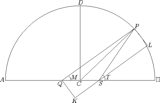 |
Let us draw the straight-line  parallel to
  , and passing through point , and then complete the rectangle
  . Simple geometry reveals that
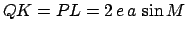 ,
,
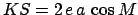 , and
, and
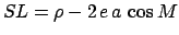 , where
 . The cosine rule applied to triangle
  yields
 , or
, or
 , which
can be solved to give
, which
can be solved to give
 .
Moreover,
.
Moreover,
 ,
which implies that
,
which implies that
![\begin{displaymath}
\frac{r}{a} = [1-2\,e\,\cos M\,(1-e^2\,\sin^2 M)^{1/2}+e^2+2\,e^2\,\sin^2 M]^{1/2}.
\end{displaymath}](img712.png) |
(87) |
Now,  , where
  is angle
  . However,
![\begin{displaymath}
\sin q = \frac{PL}{SP} = \frac{2\,e\,\sin M}{[1-2\,e\,\cos M\,(1-e^2\,\sin^2 M)^{1/2}+e^2+2\,e^2\,\sin^2 M]^{1/2}}.
\end{displaymath}](img713.png) |
(88) |
Finally, expanding the previous two equations to second-order in the small parameter , we obtain
It can be seen, by comparison with Eqs. (81)-(82) and (85)-(86), that Ptolemy's geometric model of a heliocentric planetary orbit is significantly
more accurate than Hipparchus' model, since the
relative radial distance,  , and the true anomaly, , in the former model both only deviate from those in the (correct) Keplerian model to second-order in .
Next: Model of Copernicus
Up: Geometric Planetary Orbit Models
Previous: Model of Hipparchus
Richard Fitzpatrick
2010-07-21